Logo image

Appendix B Answers to Activities

This appendix contains answers to all activities in the text. Answers for preview activities are not included.

1 Understanding the Derivative
1.1 How do we measure velocity?
1.1.2 Position and average velocity


1.1.3 Instantaneous Velocity


Activity 1.1.3.
1.1.3.b
Answer.
The instantaneous velocity at \(t = 1.5\) is approximately \(-16\) ft/sec; at \(t = 2\text{,}\) the instantaneous velocity is about \(-32\) ft/sec, and \(-16>-32\text{.}\)
1.1.3.c
Answer.
When the ball is rising, its instantaneous velocity is positive, while when the ball is falling, its instantaneous velocity is negative.


1.2 The notion of limit
1.2.2 The Notion of Limit


1.2.3 Instantaneous Velocity


Activity 1.2.4.
1.2.4.a
Answer.
\(AV_{[0.5,1]} = \frac{1-1}{1-0.5} = 0\text{,}\) \(AV_{[1.5,2.5]} = \frac{3-1}{2.5-1.5} = 2\text{,}\) and \(AV_{[0,5]} = \frac{5-0}{5-0} = 1\text{.}\)
1.2.4.b
Answer.
Take shorter and shorter time intervals and draw the lines whose slopes represent average velocity. If those lines’ slopes are approaching a single number, that number represents the instantaneous velocity.
1.2.4.c
Answer.
The instantaneous velocity at \(t = 2\) is greater than the average velocity on \([1.5,2.5]\text{.}\)

1.3 The derivative of a function at a point
1.3.2 The Derivative of a Function at a Point


Activity 1.3.3.
1.3.3.d
Answer.
described in detail following the image
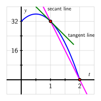
A plot of the quadratic function \(s(t) = -16t^2 + 16t + 32\text{,}\) the secant line through \((1,s(1))\) and \((2,s(2))\text{,}\) and the tangent line through \((1,s(1))\) with slope \(s'(1)=-16\)
The point \((1,32)\) is of most interest, and the curve, secant line, and tangent line all pass through this point. The function \(s(t)\) is a parabola that opens down with vertex \((\frac12,36)\) and a \(t\)-intercept at \((2,0)\text{.}\) The secant line passes through \((1,32)\) and \((2,0)\text{,}\) while the tangent line only passes through \((1,32)\text{.}\)
1.3.3.e
Answer.
\(s'(a)\) is positive whenever \(0 \le a \lt \frac{1}{2}\text{;}\) \(s'(a)\) to be negative whenever \(\frac{1}{2} \lt a \lt 2\text{;}\) \(s'(\frac{1}{2}) = 0\text{.}\)


Activity 1.3.4.
1.3.4.a
Answer.
described in detail following the image
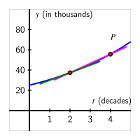
A plot of \(P(t) = 25000 e^{t/5}\) on the interval \(0 \lt t \lt 5\) (in decades). The values of \(P\) on the vertical axis range from \(0\) to \(100\) (in thousands). A secant line and a tangent line are also shown.
The function \(P(t) = 25000 e^{t/5}\) is exponential and increases as we move from left to right, beginning at the \(y\)-intercept \((0,25)\text{.}\) The points \((2,P(2))\) and \((4,P(4)\) are also shown, along with the secant line that joins those points and the tangent line to the curve at \((2,P(2))\text{.}\)
1.3.4.b
Answer.
\(AV_{[2,4]} \approx 9171\) people per decade is expected to be the average rate of change of the city’s population over the two decades from 2030 to 2050.
1.3.4.c
Answer.
\begin{equation*} P'(2) = \lim_{h \to 0} \frac{P(2+h)-P(2)}{h} = \lim_{h \to 0} 25000e^{2/5}\left( \frac{e^{h/5} - 1}{h}\right) \end{equation*}
Because there is no way to remove a factor of \(h\) from the numerator, we cannot eliminate the \(h\) that is making the denominator go to zero.
1.3.4.d
Answer.
\begin{equation*} P'(2) = \lim_{h \to 0} \frac{P(2+h)-P(2)}{h} \approx 7458.5 \end{equation*}
which is measured in people per decade.
1.3.4.e
Answer.
See the graph provided in (a). The magenta line has slope equal to the average rate of change of \(P\) on \([2,4]\text{,}\) while the green line is the tangent line at \((2,P(2))\) with slope \(P'(2)\text{.}\)
1.3.4.f
Answer.
It appears that the tangent line’s slope at the point \((a,P(a))\) will increase as \(a\) increases.

1.4 The derivative function
1.4.2 How the derivative is itself a function


1.5 Interpreting, estimating, and using the derivative
1.5.2 Units of the derivative function


Activity 1.5.2.
1.5.2.a
Answer.
\(V'(10250) = -0.89\) means that the instantaneous rate of change of the car’s value when the car has been driven \(10250\) miles is \(-0.89\) dollars per mile. In addition, when the car has been driven \(10250\) miles, if the car is driven one more mile, we expect that the value of the car will decrease by about \(0.89\) dollars.
1.5.2.b
Answer.
\(W'(0.75) = 3.43\) means that the instantaneous rate of change of volume of water in the tank when the water is \(0.75\) meters deep is \(3.43\) liters per meter. This tells us that when the water is \(0.75\) meters deep, if the water rises one more meter, we expect that the volume of water in the tank will increase by about \(3.43\) liters.
1.5.2.c
Answer.
\(S'(20) = -0.527\) means that the instantaneous rate of change of the soda’s temperature at the instant \(t = 20\) minutes is \(-0.527\) degrees Celsius per minute. This tells us that after \(20\) minutes have elapsed, if one more minute passes, we expect that the soda’s temperature will drop by about \(0.527\) degrees Celsius.
1.5.2.d
Answer.
\(C'(19) = 52.1\) means that the instantaneous rate of change of the rate at which the biker is burning calories when traveling at a speed of \(19\) kilometers per hour is \(52.1\) calories per hour per kilometer per hour. This tells us that when the person is riding at \(19\) kilometers per hour, if they increase their speed by \(1\) kilometer per hour, we expect that they will burn about \(52.1\) additional calories over the next hour.

1.5.3 Toward more accurate derivative estimates


Activity 1.5.3.
1.5.3.a
Answer.
\begin{equation*} F'(20) \approx \frac{F(30)-F(10)}{30-10} = \frac{167.6-94.7}{20} = 3.645 \end{equation*}
degrees per minute.
1.5.3.b
Answer.
\begin{equation*} F'(40) \approx \frac{F(50)-F(30)}{50-30} = \frac{197.9-167.6}{20} = 1.515 \end{equation*}
degrees per minute.
1.5.3.d
Answer.
Because at time \(t = 46\) the potato’s temperature is increasing at 1.3941 degrees per minute, we expect that at \(t = 47\text{,}\) the temperature will be about 1.3941 degrees greater than at \(t = 46\text{.}\)
1.5.3.e
Answer.
We might say that on the interval \([10,40]\)β€œthe temperature of the potato is increasing, but at a decreasing rate.”


Activity 1.5.4.
1.5.4.b
Answer.
At 80 kilometers per hour, the car is using fuel at a rate of 0.015 liters per kilometer.
1.5.4.c
Answer.
When the car is traveling at 90 kilometers per hour, its rate of fuel consumption per kilometer is increasing at a rate of 0.0006 liters per kilometer per kilometer per hour.

1.6 The second derivative
1.6.4 Concavity


Activity 1.6.2.
1.6.2.a
Answer.
Increasing: \(0\lt t\lt 2\text{,}\) \(3\lt t\lt 5\text{,}\) \(7\lt t\lt 9\text{,}\) and \(10\lt t\lt 12\text{.}\) Decreasing: never.
1.6.2.b
Answer.
Velocity is increasing on \(0\lt t\lt 1\text{,}\) \(3\lt t\lt 4\text{,}\) \(7\lt t\lt 8\text{,}\) and \(10\lt t\lt 11\text{;}\) \(y = v(t)\) is decreasing on \(1\lt t\lt 2\text{,}\) \(4\lt t\lt 5\text{,}\) \(8\lt t\lt 9\text{,}\) and \(11\lt t\lt 12\text{.}\) Velocity is constant on \(2\lt t\lt 3\text{,}\) \(5\lt t\lt 7\text{,}\) and \(9\lt t\lt 10\text{.}\)


Activity 1.6.3.
1.6.3.c
Answer.
At the moment \(t = 30\text{,}\) the temperature of the potato is \(167.6\) degrees; its temperature is rising at an instaneous rate of \(2.605\) degrees Fahrenheit per minute; and the rate at which the temperature is rising is falling at a rate of \(0.0516\) degrees Fahrenheit per minute per minute. Over the minute from \(t = 30\) to \(t = 31\text{,}\) we expect the temperature of the potato to rise about \(2.605\) degrees Fahrenheit and for the rate at which its temperature is increasing to drop by about \(0.0516\) degrees Fahrenheit per minute. We expect that \(F(31) \approx 169.7\) degrees Fahrenheit, and \(F'(31) \approx 2.01343\) degrees Fahrenheit per minute.


1.7 Limits, continuity, and differentiability
1.7.2 Having a limit at a point


Activity 1.7.2.
1.7.2.a
Answer.
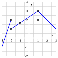
\(f(-2) = 1\text{;}\) \(f(-1)\) is not defined; \(f(0) = \frac{7}{3}\text{;}\) \(f(1) = 2\text{;}\) \(f(2) = 2\text{.}\)
1.7.2.b
Answer.
\begin{equation*} \lim_{x \to -2^-} f(x) = 2 \ \text{and} \lim_{x \to -2^+} f(x) = 1 \end{equation*}
\begin{equation*} \lim_{x \to -1^-} f(x) = \frac{5}{3} \ \text{and} \lim_{x \to -1^+} f(x) = \frac{5}{3} \end{equation*}
\begin{equation*} \lim_{x \to 0^-} f(x) = \frac{7}{3} \ \text{and} \lim_{x \to 0^+} f(x) = \frac{7}{3} \end{equation*}
\begin{equation*} \lim_{x \to 1^-} f(x) = 3 \ \text{and} \lim_{x \to 1^+} f(x) = 3 \end{equation*}
\begin{equation*} \lim_{x \to 2^-} f(x) = 2 \ \text{and} \lim_{x \to 2^+} f(x) = 2 \end{equation*}
1.7.2.c
Answer.
\(\lim_{x \to -2} f(x)\) does not exist. The values of the limits as \(x \to a\) for \(a = -1, 0, 1, 2\) are \(\frac{5}{3}, \frac{7}{3}, 3, 2\text{.}\)

1.7.3 Being continuous at a point


1.7.4 Being differentiable at a point


Activity 1.7.4.
1.7.4.b
Answer.
\begin{align*} g'(0) =\mathstrut \amp \lim_{h \to 0} \frac{g(0+h)-g(0)}{h}\\ =\mathstrut \amp \lim_{h \to 0} \frac{|0+h|-|0|}{h}\\ =\mathstrut \amp \lim_{h \to 0} \frac{|h|}{h} \end{align*}
1.7.4.c
Answer.
\(\lim_{h \to 0^+} \frac{|h|}{h} = 1 \text{,}\) but \(\lim_{h \to 0^-} \frac{|h|}{h} = -1 \text{.}\)

1.8 The tangent line approximation
1.8.3 The local linearization


Activity 1.8.2.
1.8.2.f
Answer.
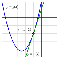
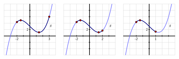
The illustration below shows a possible graph of \(y = g(x)\) near \(x = -1\text{,}\) along with the tangent line \(y = L(x)\) through \((-1, g(-1))\text{.}\)
described in detail following the image
ADD ALT TEXT TO THIS IMAGE


Activity 1.8.3.
1.8.3.e
Answer.
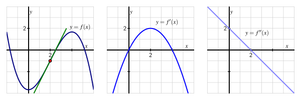
See the image below, which shows, at left, a possible graph of \(y = f(x)\) near \(x = 2\text{,}\) along with the tangent line \(y = L(x)\) through \((2, f(2))\text{.}\)
described in detail following the image
ADD ALT TEXT TO THIS IMAGE


Activity 1.8.4.
1.8.4.a
Answer.
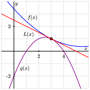
\(f(3) = 1\text{,}\) \(f'(3) = -0.5\text{,}\) \(g(3) = 1\text{,}\) and \(g'(3) = -0.5\text{;}\) this means \(f\) and \(g\) will have the same tangent line approximation at \(x = 3\text{.}\)
1.8.4.b
Answer.
\(L(x) = 1 - 0.5(x-3)\) is the tangent line approximation for both \(f\) and \(g\) at \(x = 3\text{.}\)
1.8.4.c
Answer.
\(x\) \(2.9\) \(2.99\) \(2.999\) \(3\) \(3.001\) \(3.01\) \(3.1\)
\(f(x)\) \(1.051\) \(1.00501\) \(1.0005001\) \(1\) \(0.9995001\) \(0.99501\) \(0.951\)
\(g(x)\) \(1.045\) \(1.00495\) \(1.0004995\) \(1\) \(0.9994995\) \(0.99495\) \(0.945\)
\(L(x)\) \(1.05\) \(1.005\) \(1.0005\) \(1\) \(0.9995\) \(0.995\) \(0.95\)
Near \(x = 3\text{,}\) \(L(x)\) always underestimates the value of \(f(x)\text{,}\) and \(L(x)\) always overestimates the value of \(g(x)\text{.}\)
1.8.4.d
Answer.
described in detail following the image
ADD ALT TEXT TO THIS IMAGE
Since \(f''(3) = 0.2\) ande \(g''(3)=-1\text{,}\) \(g\) has β€œmore” concavity at \(x = 3\) than \(f\text{,}\) so \(L(x)\) is a closer approximation of the value of \(f(x)\) than of the value of \(g(x)\) near \(x = 3\text{.}\)

2 Computing Derivatives
2.1 Elementary derivative rules
2.1.3 Constant, Power, and Exponential Functions


Activity 2.1.2.

2.1.4 Constant Multiples and Sums of Functions


Activity 2.1.3.


2.2 The sine and cosine functions
2.2.2 The sine and cosine functions


2.3 The product and quotient rules
2.3.2 The product rule


2.3.3 The quotient rule


Activity 2.3.3.
2.3.3.b
Answer.
\(v'(t) = \frac{(\cos(t) + t^2)\cos(t) - \sin(t)(-\sin(t) + 2t)}{(\cos(t) + t^2)^2}\text{.}\)
2.3.3.d
Answer.
\(I'(0.5) = \frac{50}{e^{0.5}} \approx 30.327\text{,}\) \(I'(2) = \frac{-100}{e^{2}} \approx -13.534\text{,}\) and \(I'(5) = \frac{-400}{e^5} \approx -2.695\text{,}\) each in candles per millisecond.
2.3.4 Combining rules


Activity 2.3.4.
2.3.4.a
Answer.
\(f'(r) = (5r^3 + \sin(r))[4^r \ln(4) + 2\sin(r)] + (4^r - 2\cos(r))[15r^2 + \cos(r)]\text{.}\)
2.3.4.b
Answer.
\(p'(t) = \frac{t^6 \cdot 6^t [-\sin(t)] - \cos(t) [t^6 \cdot 6^t \ln(6) + 6^t \cdot 6t^5]}{(t^6 \cdot 6^t)^2}\text{.}\)
2.3.4.c
Answer.
\(g'(z) = 3 [z^7 e^z + 7z^6e^z] - 2[z^2 \cos(z) + 2z\sin(z)] + \frac{(z^2+1) 1 - z(2z)}{(z^2 + 1)^2}\text{.}\)

2.4 Derivatives of other trigonometric functions
2.4.2 Derivatives of the cotangent, secant, and cosecant functions


Activity 2.4.4.
2.4.4.b
Answer.
\(p'(\frac{\pi}{4}) = \frac{\pi^2}{16} \sqrt{2} + \frac{\sqrt{2}\pi}{2} + \frac{\pi}{2} - 1\text{.}\)
2.4.4.c
Answer.
\(h'(t) = \frac{(t^2+1) \sec^2(t) - 2t \tan(t)}{(t^2 + 1)^2} + 2e^t \sin(t) - 2 e^t\cos(t)\text{.}\)

2.5 The chain rule
2.5.2 The chain rule


2.5.3 Using multiple rules simultaneously


Activity 2.5.3.
2.5.3.c
Answer.
\(h'(y) = \frac{(e^{4y}+1) [-10\sin(10y)] - \cos(10y) [4e^{4y}]}{(e^{4y}+1)^2}\text{.}\)
2.5.3.d
Answer.
\(s'(z) = 2^{z^2\sec(z)} \ln(2) [z^2 \sec(z)\tan(z) + \sec(z) \cdot 2z]\text{.}\)


2.6 Derivatives of inverse functions
2.6.3 The derivative of the natural logarithm function


2.6.4 Inverse trigonometric functions and their derivatives


Activity 2.6.4.
2.6.4.a
Answer.
\(f'(x) = \left[x^3 \cdot \frac{1}{1+x^2} + \arctan(x) \cdot 3x^2 \right] + \left[e^x \cdot \frac{1}{x} + \ln(x) \cdot e^x\right]\text{.}\)
2.6.4.b
Answer.
\(p'(t) = 2^{t\arcsin(t)} \ln(2) [t \cdot \frac{1}{\sqrt{1-t^2}} + \arcsin(t) \cdot 1]\text{.}\)
2.6.4.c
Answer.
\(h'(z) = 27(\arcsin(5z) + \arctan(4-z))^{26} \left[\frac{1}{\sqrt{1-(5z)^2}} \cdot 5 + \frac{1}{1+(4-z)^2} \cdot (-1) \right]\text{.}\)
2.6.4.f
Answer.
\(g'(w) = \frac{1}{1+ \left( \frac{\ln(w)}{1+w^2} \right)^2} \cdot \left[ \frac{(1+w^2) \frac{1}{w} - \ln(w) \cdot 2w}{(1+w^2)^2} \right] \)

2.7 Derivatives of functions given implicitly
2.7.2 Implicit Differentiation


Activity 2.7.3.
2.7.3.a
Answer.
Horizontal at \(x \approx 0.42265\text{,}\) thus \((0.42265, -1.05782); (0.42265, 0.229478); (0.42265, 0.770522); (0.42265, 2.05782)\text{.}\) There are four more points where \(x \approx 1.57735\text{.}\)
2.7.3.b
Answer.
When \(y = \frac{1}{2}, \frac{1 \pm \sqrt{5}}{2}\text{,}\) so one point is \((2.21028, \frac{1}{2})\text{.}\)


Activity 2.7.4.
2.7.4.a
Answer.
\(\frac{dy}{dx}(-3y^2 - 6x) = 6y-3x^2 \) and the tangent line has equation \(y - 3 = 1(x+3)\text{.}\)
2.7.4.b
Answer.
\(\frac{dy}{dx} = \frac{3x^2 + 1}{\cos(y) + 1}\) and the tangent line has equation \(y = \frac{1}{2}x\text{.}\)
2.7.4.c
Answer.
\(\frac{dy}{dx} = \frac{3e^{-xy} - 3xye^{-xy}}{3x^2e^{-xy}+2y}\) and the tangent line is \(y - 1 = 0.234950(x - 0.619061)\text{.}\)

3 Using Derivatives
3.1 Related rates
3.1.2 Related Rates Problems


Activity 3.1.2.
3.1.2.e
Answer.
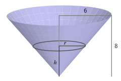
\(\left. \frac{dh}{dt} \right|_{h=3} = \frac{64}{81\pi} \approx 0.2515\) feet per minute.


Activity 3.1.5.
Answer.
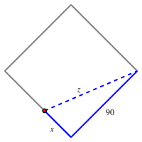
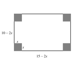
Let \(x\) denote the position of the ball at time \(t\) and \(z\) the distance from the ball to first base, as pictured below.
described in detail following the image
ADD ALT TEXT TO THIS IMAGE
\(\left. \frac{dz}{dt} \right|_{x = 45} = \frac{100}{\sqrt{5}} \approx 44.7214 \ \text{feet/sec} \text{.}\)
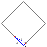
Let \(r\) be the runner’s position at time \(t\) and let \(s\) be the distance between the runner and the ball, as pictured.
described in detail following the image
ADD ALT TEXT TO THIS IMAGE
\(\left. \frac{ds}{dt} \right|_{x = 45} = \frac{430}{\sqrt{17}} \approx 104.2903 \ \text{feet/sec} \text{.}\)

3.2 Using derivatives to evaluate limits
3.2.2 Using derivatives to evaluate indeterminate limits of the form \(\frac{0}{0}\text{.}\)


3.2.3 Limits involving \(\infty\)


Activity 3.2.4.
3.2.4.d
Answer.
\(\lim_{x \to \frac{\pi}{2}^-} \frac{\tan(x)}{x-\frac{\pi}{2}} = -\infty\text{.}\)

3.3 Using derivatives to identify extreme values
3.3.2 Critical numbers and the first derivative test


Activity 3.3.2.
3.3.2.b
Answer.
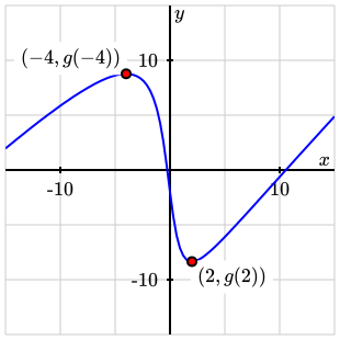
For \(x \lt -4\text{,}\) \(g'(x) \gt 0\text{;}\) for \(-4 \lt x \lt 2\text{,}\) \(g'(x) \lt 0\text{;}\) and for \(x \gt 2\text{,}\) \(g'(x) \gt 0\text{.}\)
3.3.2.c
Answer.
\(g\) has a local maximum at \(x = -4\text{;}\) \(g\) has a local minimum at \(x = 2\text{.}\)
3.3.2.d
Answer.
described in detail following the image
A plot of a possible function \(y = g(x)\) whose derivative is the given formula for \(g'(x)\text{.}\)
Figure 3.3.8. A plot of a possible function \(y = g(x)\) whose derivative is the given formula for \(g'(x)\text{.}\)

3.3.3 The second derivative test


Activity 3.3.4.
3.3.4.a
Answer.
In the graph below, \(h(x) = x^2 + \cos(3x)\) is given in dark blue, while \(h(x) = x^2 + \cos(1.6x)\) is shown in light blue.
3.3.4.b
Answer.
If \(\frac{2}{k^2} \gt 1\text{,}\) then the equation \(\cos(kx) = \frac{2}{k^2}\) has no solution. Hence, whenever \(k^2 \lt 2\text{,}\) or \(k \lt \sqrt{2} \approx 1.414\text{,}\) it follows that the equation \(\cos(kx) = \frac{2}{k^2}\) has no solutions \(x\text{,}\) which means that \(h''(x)\) is never zero (indeed, for these \(k\)-values, \(h''(x)\) is always positive so that \(h\) is always concave up). On the other hand, if \(k \ge \sqrt{2}\text{,}\) then \(\frac{2}{k^2} \le 1\text{,}\) which guarantees that \(\cos(kx) = \frac{2}{k^2}\) has infinitely many solutions, due to the periodicity of the cosine function. At each such point, \(h''(x) = 2 - k^2 \cos(kx)\) changes sign, and therefore \(h\) has infinitely many inflection points whenever \(k \ge \sqrt{2}\text{.}\)
3.3.4.c
Answer.
To see why \(h\) can only have a finite number of critical numbers regardless of the value of \(k\text{,}\) consider the equation
\begin{equation*} 0 = h'(x) = 2x - k\sin(kx)\text{,} \end{equation*}
which implies that \(2x = k\sin(kx)\text{.}\) Since \(-1 \le \sin(kx) \le 1\text{,}\) we know that \(-k \le k\sin(kx) \le k\text{.}\) Once \(|x|\) is sufficiently large, we are guaranteed that \(|2x| \gt k\text{,}\) which means that for large \(x\text{,}\) \(2x\) and \(k\sin(kx)\) cannot intersect. Moreover, for relatively small values of \(x\text{,}\) the functions \(2x\) and \(k\sin(kx)\) can only intersect finitely many times since \(k\sin(kx)\) oscillates a finite number of times. This is why \(h\) can only have a finite number of critical numbers, regardless of the value of \(k\text{.}\)

3.4 Using derivatives to describe families of functions
3.4.2 Describing families of functions in terms of parameters


Activity 3.4.2.
3.4.2.a
Answer.
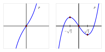
\(p\) has two critical numbers (\(x = \pm \sqrt{\frac{a}{3}}\)) whenever \(a \gt 0\) and no critical numbers when \(a \lt 0\text{.}\)
3.4.2.b
Answer.
When \(a \lt 0\text{,}\) \(p\) is always increasing and has no relative extreme values. When \(a\gt 0\text{,}\) \(p\) has a relative maximum at \(x = -\sqrt{\frac{a}{3}}\) and a relative minimum at \(x = +\sqrt{\frac{a}{3}}\text{.}\)
3.4.2.c
Answer.
\(p\) is CCD for \(x \lt 0\) and \(p\) is CCU for \(x\gt 0\text{,}\) making \(x = 0\) an inflection point.


Activity 3.4.3.
3.4.3.c
Answer.
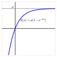
\(\lim_{x \to \infty} a(1-e^{-bx}) = a\text{,}\) and \(\lim_{x \to \infty} a(1-e^{-bx}) = -\infty\text{.}\)
3.4.3.d
Answer.
If \(b\) is large and \(x\) is close to zero, \(h'(x)\) is relatively large near \(x = 0\text{,}\) and the curve’s slope will quickly approach zero as \(x\) increases. If \(b\) is small, the graph is less steep near \(x = 0\) and its slope goes to zero less quickly as \(x\) increases.


Activity 3.4.4.
3.4.4.b
Answer.
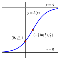
\(L\) is concave up for all \(t \lt -\frac{1}{k} \ln \left(\frac{1}{c}\right)\) and concave up for all other values of \(t\text{.}\)
3.4.4.c
Answer.
\(\lim_{t \to \infty} \frac{A}{1+ce^{-kt}} = A\text{,}\) and
\begin{equation*} \lim_{t \to \infty} \frac{A}{1+ce^{-kt}} = 0\text{.} \end{equation*}
3.4.4.d
Answer.
The inflection point on the graph of \(L\) is \(( -\frac{1}{k} \ln \left(\frac{1}{c}\right), \frac{A}{2})\text{.}\)

3.5 Global optimization
3.5.2 Global Optimization


Activity 3.5.2.
3.5.2.c
Answer.
On \([-2,3]\text{,}\) \(g\) has a global maximum at \(x = 3\) and a global minimum at \(x = \sqrt{2}\text{.}\)
3.5.2.d
Answer.
On \([-2,2]\text{,}\) \(g\) has a global maximum at \(x = -\sqrt{2}\) and a global minimum at \(x = \sqrt{2}\text{.}\)
3.5.2.e
Answer.
On \([-2,1]\text{,}\) \(g\) has a global maximum at \(x = -\sqrt{2}\) and a global minimum at \(x = 1\text{.}\)


Activity 3.5.3.

3.5.3 Moving toward applications


Activity 3.5.4.

3.6 Applied optimization
3.6.2 More applied optimization problems


Activity 3.6.2.
3.6.2.b
Answer.
\(V = \pi r^2 h\text{;}\) \(S = 2 \pi r^2 + 2 \pi r h\text{;}\) \(C = 2 \pi r^2 \cdot 0.027 + 2 \pi r h \cdot 0.015\text{.}\)
3.6.2.d
Answer.
\(r = \sqrt[3]{ \frac{0.48}{0.108 \pi} } \approx 1.12259\text{;}\) \(h \approx 4.041337\text{;}\) minimum cost \(C(1.12259) \approx 0.64137\text{.}\)


Activity 3.6.3.
Answer.
The absolute minimum time the hiker can achieve is \(0.99302\) hours, which is attained by hiking about 2.2 km from \(P\) to \(Q\) and then turning into the woods for the remainder of the trip.


Activity 3.6.4.
Answer.
\(A(1.19606) \approx 2.2018\) is the absolute maximum cross-sectional area, which leads to the absolute maximum volume.


Activity 3.6.5.
Answer.
Maximum area: \(A(\frac{5}{\sqrt{3}}) = \frac{500}{9}\sqrt{3} \approx 96.225\text{.}\) Maximum perimeter: \(P(1) = 52\text{.}\)

4 The Definite Integral
4.1 Determining distance traveled from velocity
4.1.2 Area under the graph of the velocity function


Activity 4.1.2.
4.1.2.a
Answer.
\begin{align*} A =\mathstrut \amp v(0.0) \cdot 0.5 + v(0.5) \cdot 0.5 + v(1.0) \cdot 0.5 + v(1.5) \cdot 0.5\\ =\mathstrut \amp 1.500 \cdot 0.5 + 1.9375 \cdot 0.5 + 2.000 \cdot 0.5 + 2.0625 \cdot 0.5\\ =\mathstrut \amp 3.75 \end{align*}
Thus, \(D \approx 3.75\) miles.
4.1.2.c
Answer.
\(s(t) = \frac{1}{8}t^4 - \frac{1}{2} t^3 + \frac{3}{4} t^2 + \frac{3}{2}t\text{.}\)
4.1.2.d
Answer.
\(s(2) - s(0) = \frac{1}{8}2^4 - \frac{1}{2}2^3 + \frac{3}{4}2^2 + \frac{3}{2} 2 = 4\text{.}\)

4.1.3 Two approaches: area and antidifferentiation


Activity 4.1.3.
4.1.3.d
Answer.
\(A = 4\) feet is the total distance the ball traveled vertically on \([\frac{1}{2},1]\text{.}\)
4.1.3.e
Answer.
\(s(1) - s(0) = 16\) is the vertical distance the ball traveled on the interval \([0,1]\text{.}\) Equivalently, the area between the velocity curve and the \(t\)-axis on \([0,1]\) is \(A = 16\) feet.
4.1.3.f
Answer.
\(s(2) - s(0) = 0\text{,}\) so the ball has zero change in position on the interval \([0,2]\text{.}\)

4.1.4 When velocity is negative


4.2 Riemann sums
4.2.2 Sigma Notation


4.2.3 Riemann Sums


4.2.4 When the function is sometimes negative


4.3 The definite integral
4.3.2 The definition of the definite integral


4.3.3 Some properties of the definite integral


4.3.4 How the definite integral is connected to a function’s average value


Activity 4.3.4.
4.3.4.a
Answer.
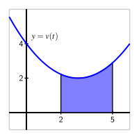
\(y = v(t) = \sqrt{4-(t-2)^2}\) is the top half of the circle \((t-2)^2 + y^2 = 4\text{,}\) which has radius 2 and is centered at \((2,0)\text{.}\)
4.3.4.e
Answer.
The height of the rectangle is the average value of \(v\text{,}\) \(v_{\text{AVG} }[0,4] = \frac{\pi}{2} \approx 1.57\text{.}\)

4.4 The Fundamental Theorem of Calculus
4.4.2 The Fundamental Theorem of Calculus


4.4.3 Basic antiderivatives


Activity 4.4.3.
4.4.3.a
Answer.
given function, \(f(x)\) antiderivative, \(F(x)\) Β 
\(k\text{,}\) (\(k \ne 0\)) \(kx\)
\(x^n\text{,}\) \(n \ne -1\) \(\frac{1}{n+1}x^{n+1}\)
\(\frac{1}{x}\text{,}\) \(x \gt 0\) \(\ln(x)\)
\(\sin(x)\) \(-\cos(x)\)
\(\cos(x)\) \(\sin(x)\)
\(\sec(x) \tan(x)\) \(\sec(x)\)
\(\csc(x) \cot(x)\) \(-\csc(x)\)
\(\sec^2 (x)\) \(\tan(x)\)
\(\csc^2 (x)\) \(-\cot(x)\)
\(e^x\) \(e^x\)
\(a^x\) \((a \gt 1)\) \(\frac{1}{\ln(a)} a^x\)
\(\frac{1}{1+x^2}\) \(\arctan(x)\)
\(\frac{1}{\sqrt{1-x^2}}\) \(\arcsin(x)\)
\(\int_0^1 \left(x^3 - x - e^x + 2\right) \,dx = \frac{11}{4} - e\text{.}\)
4.4.3.b
Answer.
\(\int_0^{\pi/3} (2\sin (t) - 4\cos(t) + \sec^2(t) - \pi) \, dt = 1 - \sqrt{3} - \frac{\pi^2}{3}\text{.}\)

4.4.4 The total change theorem


Activity 4.4.4.
4.4.4.a
Answer.
The person burned exactly \(\frac{400}{3}\) calories in the first 10 minutes of the workout.
4.4.4.b
Answer.
\(C(40) - C(0) = \int_0^{40} C'(t) \, dt = \int_0^{40} c(t) \, dt\) is the total calories burned on \([0,40]\text{.}\)
4.4.4.c
Answer.
The exact average rate at which the person burned calories on \(0 \le t \le 40\) is
\begin{equation*} c_{\operatorname{AVG} [0,40]} = \frac{1}{40-0} \int_0^{40} c(t) \, dt = \frac{1}{40} \cdot \frac{1700}{3} = \frac{1700}{120} \approx 14.17 \ \text{cal/min}\text{.} \end{equation*}
4.4.4.d
Answer.
One time at which the instantaneous rate at which calories are burned equals the average rate on \([0,40]\) is \(t = \frac{5}{3}(6 - \sqrt{6}) \approx 5.918\text{.}\)

5 Evaluating Integrals
5.1 Constructing accurate graphs of antiderivatives
5.1.2 Constructing the graph of an antiderivative


Activity 5.1.2.
5.1.2.a
Answer.
\(F\) is increasing on \((0,2)\) and \((5,7)\text{;}\) \(F\) is decreasing on \((2,5)\text{.}\)
5.1.2.b
Answer.
\(F\) is concave up on \((0,1)\text{,}\) \((4,6)\text{;}\) concave down on \((1,3)\text{,}\) \((6,7)\text{;}\) neither on \((3,4)\text{.}\)
5.1.2.d
Answer.
\(F(1) = -\frac{1}{2}\text{;}\) \(F(2) = \frac{\pi}{4} - \frac{1}{2}\text{;}\) \(F(3) = \frac{\pi}{4} - 1\text{;}\) \(F(4) = \frac{\pi}{4}-2\text{;}\) \(F(5) = \frac{\pi}{4} - \frac{5}{2}\text{;}\) \(F(6) = \frac{\pi}{2} - \frac{5}{2}\text{;}\) \(F(7) = \frac{3\pi}{4} - \frac{5}{2}\text{;}\) \(F(8) = \frac{3\pi}{4} - \frac{5}{2}\text{;}\) and \(F(-1) = -1\text{.}\)
5.1.2.e
Answer.
Use the function values found in (d) and the earlier information regarding the shape of \(F\text{.}\)

5.1.3 Multiple antiderivatives of a single function


Activity 5.1.3.
5.1.3.a
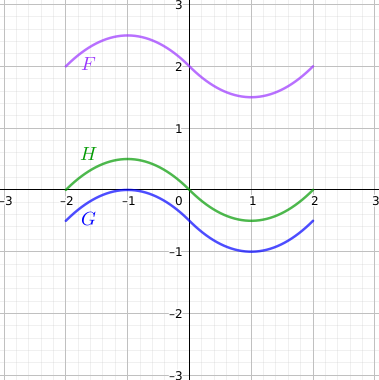
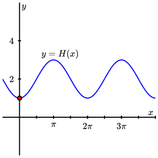
Answer.
described in detail following the image
This image shows three possible antiderivatives of \(g(x)\) on the interval \([-2,2]\text{.}\)
The first, \(G(x)\text{,}\) looks like two quadratic functions joined together at \(x = 0\text{:}\) one that’s concave down on the left, and another that’s concave up on the right. Three important points on the graph of \(G(x)\) are \(G(-1) = 0\text{,}\) \(G(0) = -\frac12\text{,}\) and \(G(1) = -1\text{.}\)
The other two antiderivatives, \(H(x)\) and \(F(x)\text{,}\) are vertical shifts of \(G(x)\text{.}\) \(H(x)\) satisfies \(H(-2)=0\) and \(F(x)\) satisfies \(F(-2)=2\text{.}\)
5.1.3.b
Answer.
described in detail following the image
Plot of the antiderivative \(H(x)\) that satisfies the prescribed conditions.
Figure 5.1.3. Plot of \(H(x)\text{.}\)
5.1.3.c
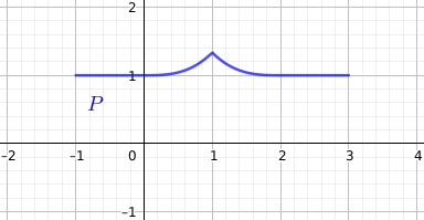
Answer.
described in detail following the image
This image shows the described antiderivative \(P(x)\) on the interval \([-1,3]\text{.}\)
On the intervals \([-1,0]\) and \([2,3]\text{,}\) \(P(x)=0\text{.}\) On the interval \((0,1)\text{,}\) \(P(x)\) is increasing and concave up. There’s a corner point on the graph of \(P(x)\) at the point \((1,4/3)\text{,}\) and there \(P(x)\) changes to become decreasing and concave up on the interval \((1,2)\text{.}\)

5.1.4 Functions defined by integrals


Activity 5.1.4.
5.1.4.a
Answer.
\(A\) is increasing on \((0,1.5)\text{,}\) \((4,6)\text{;}\) \(A\) is decreasing on \((1.5,4)\text{.}\)
5.1.4.b
Answer.
\(A\) is concave up on \((0,1)\) and \((3,5)\text{;}\) \(A\) is concave down on \((1,3)\) and \((5,6)\text{.}\)
5.1.4.c
Answer.
At \(x = 1.5\text{,}\) \(A\) has a relative maximum; \(A\) has a relative minimum at \(x = 4\text{.}\)
5.1.4.d
Answer.
\(A(0) = -\frac{1}{2}\text{;}\) \(A(1) = 0\text{;}\) \(A(2) = 0\text{;}\) \(A(3) = -2\text{;}\) \(A(4) = -3.5\text{,}\) \(A(5) = -2\text{,}\) \(A(6) = -0.5\text{.}\)

5.2 The Second Fundamental Theorem of Calculus
5.2.2 The Second Fundamental Theorem of Calculus


Activity 5.2.2.
5.2.2.c
Answer.
\(A\) is increasing wherever \(f\) is positive; \(A\) is CCU wherever \(f\) is increasing. \(A(2) = 0\text{,}\) \(A(3) = -0.5\text{,}\) \(A(4) = -1.5\text{,}\) \(A(5) = -2\text{,}\) \(A(6) = -2 + \frac{\pi}{4}\text{,}\) and \(A(7) = -2 + \frac{\pi}{2}\text{.}\)
5.2.2.e
Answer.
\(B\) and \(C\) have the same shape as \(A\) and \(F\text{,}\) and differ from \(A\) by a constant. Observe that \(B(3) = 0\) and \(C(1) = 0\text{.}\)

5.2.3 Understanding Integral Functions


Activity 5.2.3.
5.2.3.b
Answer.
\(F\) is increasing for all \(x \gt 0\text{;}\) \(F\) is decreasing for \(x \lt 0\)
5.2.3.c
Answer.
\(F\) is CCU on \(-1 \lt x \lt 1\) and CCD for \(x \lt -1\) and \(x \gt 1\text{.}\)
5.2.3.d
Answer.
\(x\) \(-10\) \(-5\) \(0\) \(5\) \(10\)
\(F(x)\) 2.35973 1.64038 0 1.64038 2.35973
5.2.3.e
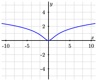
Answer.
described in detail following the image
A plot of \(y = F(x)\text{.}\) The \(x\) values on the coordinate axes range horizontally from \(-10.5\) to \(-10.5\text{,}\) and the \(y\) values range vertically from \(-5.5\) to \(-5.5\text{.}\) The function \(F\) is decreasing for \(x \lt 0\) and increasing for \(x \gt 0\) with a global minimum at \(x = 0\text{.}\) The function \(F\) is concave up for approximately \(-1 \lt x \lt 1\) and concave down otherwise.

5.2.4 Differentiating an Integral Function


Activity 5.2.4.
5.2.4.a
Answer.
\(\displaystyle \frac{d}{dx} \left[ \int_4^x e^{t^2} \, dt \right] = e^{x^2}\text{.}\)
5.2.4.b
Answer.
\(\displaystyle \int_{-2}^x \frac{d}{dt} \left[ \frac{t^4}{1+t^4} \right] \, dt = \frac{x^4}{1+x^4} - \frac{16}{17}\text{.}\)
5.2.4.c
Answer.
\(\displaystyle \frac{d}{dx} \left[ \int_{x}^1 \cos(t^3) \, dt \right] = -\cos(x^3)\text{.}\)
5.2.4.d
Answer.
\(\displaystyle \int_{3}^x \frac{d}{dt} \left[ \ln(1+t^2) \right] \, dt = \ln(1+x^2)-\ln(10)\text{.}\)
5.2.4.e
Answer.
\(\displaystyle \frac{d}{dx} \left[ \int_4^{x^3} \sin(t^2) \, dt \right] = \sin(x^6) \cdot 3x^2\text{.}\)

5.3 Integration by substitution
5.3.2 Reversing the Chain Rule: First Steps


Activity 5.3.2.
5.3.2.c
Answer.
\(\displaystyle \int \frac{1}{11x - 9} \, dx = \frac{1}{11} \ln|11x - 9| + C\text{.}\)
5.3.2.d
Answer.
\(\displaystyle \int \csc(2x+1) \cot(2x+1) \, dx = -\frac{1}{2}\csc(2x+1) + C\text{.}\)
5.3.2.e
Answer.
\(\displaystyle \int \frac{1}{\sqrt{1-16x^2}}\, dx = \frac{1}{4} \arcsin(4x) + C\)

5.3.3 Reversing the Chain Rule: \(u\)-substitution


5.3.4 Evaluating Definite Integrals via \(u\)-substitution


Activity 5.3.4.
5.3.4.a
Answer.
\(\displaystyle \int_{x=1}^{x=2} \frac{x}{1 + 4x^2} \, dx = \frac{1}{8} (\ln(17) - \ln(5))\text{.}\)
5.3.4.b
Answer.
\(\displaystyle \int_0^1 e^{-x} (2e^{-x}+3)^{9} \, dx = -\frac{1}{20}(2e^{-1}+3)^{10} + \frac{1}{20}(2e^{0}+3)^{10}\text{.}\)
5.3.4.c
Answer.
\(\displaystyle \int_{2/\pi}^{4/\pi} \frac{\cos\left(\frac{1}{x}\right)}{x^{2}} \,dx = 1 - \frac{\sqrt{2}}{2}\text{.}\)

5.4 Integration by parts
5.4.2 Reversing the Product Rule: Integration by Parts


5.4.3 Some Subtleties with Integration by Parts


Activity 5.4.3.
5.4.3.a
Answer.
\(\displaystyle \int{\arctan(x) dx} = x\arctan(x) - \frac{1}{2} \ln \left( | 1 + x^2 | \right) + c \text{.}\)
5.4.3.c
Answer.
\(\displaystyle \int t^3 \sin(t^2) dt = \frac{1}{2} \left( -t^2 \cos\left(t^2 \right) + \sin\left(t^2\right) \right) + C \text{.}\)
5.4.3.d
Answer.
\(\int s^5 e^{s^3} ds = \frac{1}{3} \left( s^3 e^{s^3} - e^{s^3} \right) + c \text{.}\)
5.4.3.e
Answer.
\(\int e^{2t} \cos\left( e^t \right) dt = e^t \sin \left( e^t \right) + \cos \left( e^t \right) + c \text{.}\)

5.4.4 Using Integration by Parts Multiple Times


Activity 5.4.4.
5.4.4.a
Answer.
\(\displaystyle \int x^2 \sin(x) dx = -x^2 \cos(x) + 2x \sin(x) + 2 \cos(x) + c \text{.}\)
5.4.4.b
Answer.
\(\displaystyle \int t^3 \ln(t) dt = \frac{1}{4} t^4 \ln(t) - \frac{1}{16} t^4 + c \text{.}\)
5.4.4.c
Answer.
\(\displaystyle \int e^z \sin(z) dz = -\frac{1}{2}e^z \cos(z) + \frac{1}{2}e^z \sin(z) + c \text{.}\)
5.4.4.d
Answer.
\(\displaystyle \int s^2 e^{3s} ds = \frac{1}{3}s^2 e^{3s} - \frac{2}{9}s e^{3s} + \frac{2}{27} e^{3s} + c \text{.}\)
5.4.4.e
Answer.
\(\displaystyle \int t \arctan(t) dt = \frac{1}{2}t^2 \arctan(t) - \frac{1}{2}t + \frac{1}{2} \arctan(t) + c \text{.}\)

5.5 Other options for finding algebraic antiderivatives
5.5.2 The Method of Partial Fractions


Activity 5.5.2.
5.5.2.a
Answer.
\(\displaystyle \int \frac{1}{x^2 - 2x - 3} \, dx = \frac{1}{4}\ln|x-3| - \frac{1}{4}\ln|x+1| + C\text{.}\)
5.5.2.b
Answer.
\(\displaystyle \int \frac{x^2+1}{x^3 - x^2} \, dx = -\ln|x| + x^{-1} + 2\ln|x-1| + C\text{.}\)
5.5.2.c
Answer.
\(\displaystyle \int \frac{x-2}{x^4 + x^2}\, dx = \ln|x| + 2x^{-1} - \frac{1}{2} \ln|1+x^2| + 2\arctan(x) + C\text{.}\)

5.5.3 Using an Integral Table


Activity 5.5.3.
5.5.3.a
Answer.
\(\displaystyle \int \sqrt{x^2 + 4} \, dx = \frac{x}{2} \sqrt{x^2+4} + 2 \ln | x + \sqrt{x^2+4}| + C\text{.}\)
5.5.3.b
Answer.
\(\displaystyle \int \frac{x}{\sqrt{x^2 +4}} \, dx = \sqrt{x^2 + 4} + C\text{.}\)
5.5.3.c
Answer.
\(\displaystyle \int \frac{2}{\sqrt{16+25x^2}}\, dx = \frac{2}{5} \ln| 5x + \sqrt{16+25x^2} | + C\text{.}\)
5.5.3.d
Answer.
\(\displaystyle \int \frac{1}{x^2 \sqrt{49-36x^2}} \, dx = - \frac{\sqrt{49-36x^2}}{49x} + C\text{.}\)

5.6 Numerical integration
5.6.2 The Trapezoid Rule


Activity 5.6.2.
5.6.2.b
Answer.
The table below gives values of the trapezoid rule and corresponding errors for different \(n\)-values.
\(n\) \(T_n\) \(E_{T,n}\)
\(4\) \(0.50899\) \(0.00899\)
\(8\) \(0.50227\) \(0.00227\)
\(16\) \(0.50057\) \(0.00057\)
5.6.2.c
Answer.
The table below gives values of the midpoint rule and corresponding errors for different \(n\)-values.
\(n\) \(M_n\) \(E_{M,n}\)
\(4\) \(0.49555\) \(-0.00445\)
\(8\) \(0.49887\) \(-0.00113\)
\(16\) \(0.49972\) \(-0.00028\)

5.6.4 Simpson’s Rule


Activity 5.6.3.
5.6.3.c
Answer.
\begin{align*} L_3 \amp = 165.6 \text{ ft } \amp R_3 \amp = 105.6 \text{ ft } \amp T_3 \amp = 135.6 \text{ ft}\text{.} \end{align*}
\(R_3\) and \(T_3\) are underestimates.
5.6.3.f
Answer.
Simpson’s rule gives the best approximation of the distance traveled, \(\int_0^{1.8} v(t) dt \approx 140.8 \text{ ft}\text{,}\) which leads to \(AV_{[0,1.8]} \approx \frac{140.8}{1.8} \approx 78.22 \text{ ft/sec}\text{.}\)

5.6.5 Overall observations regarding \(L_n\text{,}\) \(R_n\text{,}\) \(T_n\text{,}\) \(M_n\text{,}\) and \(S_{2n}\text{.}\)


Activity 5.6.4.
5.6.4.a
Answer.
\(L_1 = 2\) for each of the three functions and \(R_1 = 1\) for each.
The values of \(L_1\) and \(R_1\) are the same for all three.
5.6.4.b
Answer.
For \(f\text{,}\) \(g\text{,}\) and \(h\text{,}\) respectively, \(M_1 = 7/4\text{,}\) \(15/8\text{,}\) and \(31/16\text{.}\)
5.6.4.d
Answer.
\begin{align*} \int_0^1 f(x) dx \amp = \frac{5}{3} \amp \int_0^1 g(x) dx \amp = \frac{7}{4} \amp \int_0^1 h(x) dx \amp = \frac{9}{5} \end{align*}
5.6.4.e
Answer.
Left endpoint rule results are overestimates; right endpoint rules are underestimates; midpoint rules are overestimates; trapezoid rules are underestimates. Simpson’s rule is exact for both \(f\) and \(g\text{,}\) while a slight underestimate of \(\int_0^1 h(x) dx\text{.}\)

6 Using Definite Integrals
6.1 Using definite integrals to find area and length
6.1.2 The Area Between Two Curves


Activity 6.1.2.
6.1.2.b
Answer.
\(A = \int_{-\sqrt{20}/3}^{\sqrt{20}/3} ((12-2x^2)-(x^2-8)) \, dx \frac{160 \sqrt{\frac{5}{3}}}{3} \approx 68.853\text{.}\)
6.1.2.c
Answer.
\(A = \int_0^\frac{\pi}{4} \left( \cos(x) - \sin(x) \right) dx = \sqrt{2} - 1\text{.}\)
6.1.2.d
Answer.
The left-hand region has area
\begin{equation*} A_1 = \int_{\frac{1 - \sqrt{5}}{2}}^0 \left( \left(x^3 - x \right) - x^2\right) dx = \dfrac{13 - 5\sqrt{5}}{24} \approx 0.075819\text{.} \end{equation*}
The right-hand region has area
\begin{equation*} A_2 = \int_0^{\frac{1 + \sqrt{5}}{2}} \left( x^2 - \left(x^3 - x \right) \right) dx = \dfrac{13 + 5\sqrt{5}}{24} \approx 1.007514 \text{.} \end{equation*}
The total area is \(A_1 + A_2 \approx 1.083333\text{.}\)

6.1.3 Finding Area with Horizontal Slices


6.1.4 Finding the length of a curve


Activity 6.1.4.
6.1.4.d
Answer.
We will usually have to estimate the value of \(\int_a^b \sqrt{1+f'(x)^2} \, dx\) using computational technology.

6.2 Using definite integrals to find volume
6.2.2 The Volume of a Solid of Revolution


Activity 6.2.2.
6.2.2.b
Answer.
\(V = \int_0^4 \pi (4-(\sqrt{x})^2) \, dx = \int_0^4 \pi (4-x) \, dx = 8\pi\text{.}\)
6.2.2.d
Answer.
\(V = \int_{-\sqrt{3}}^{\sqrt{3}} \pi( (x^2 + 4)^2 - (2x^2 + 1)^2) \, dx = \frac{136\sqrt{3}}{5}\pi\text{.}\)

6.2.3 Revolving about the \(y\)-axis


6.2.4 Revolving about horizontal and vertical lines other than the coordinate axes


Activity 6.2.4.
6.2.4.a
Answer.
\begin{equation*} V = \int_{0}^{\sqrt{2}} \pi ( (2x+2)^2 - (x^3 + 2)^2 ) \, dx = \frac{4}{21}(21+8\sqrt{2}) \pi \approx 19.336\text{.} \end{equation*}
6.2.4.b
Answer.
\begin{equation*} V = \int_{0}^{\sqrt{2}} \pi ( (4 - x^3)^2 - (4-2x)^2 ) \, dx = \left( 8-\frac{32\sqrt{2}}{21} \right)\pi \approx 18.3626\text{.} \end{equation*}
6.2.4.c
Answer.
\begin{equation*} V = \int_{0}^{2\sqrt{2}} \pi( (y^{1/3} + 1)^2 - (\frac{1}{2}y + 1)^2 ) \, dy = \frac{2}{15}(15 + 8\sqrt{2}) \pi \approx 11.022\text{.} \end{equation*}
6.2.4.d
Answer.
\begin{equation*} V = \int_{0}^{2\sqrt{2}} \pi( (5 - \frac{1}{2}y)^2 - (5 - y^{1/3})^2 ) \, dy = \frac{2}{15}(75-8\sqrt{2})\pi \approx 26.677\text{.} \end{equation*}

6.3 Density, mass, and center of mass
6.3.2 Density


Activity 6.3.2.
6.3.2.b
Answer.
  1. \(V = \int_{0}^{5} \pi (4 - \frac{4}{5}x)^2 \, dx = \frac{80\pi}{3} \approx 83.7758 \mbox{m}^3\text{.}\)
  2. \(M = \frac{64000\pi}{3} \approx 67020.6433 \mbox{kg} \text{.}\)
  3. \(\displaystyle M = \int_{0}^{5} (400 + \frac{200}{1+x^2}) \cdot \pi (4-\frac{4}{5}x)^2 \, dx = 128 \pi (\frac{265}{3} + 24 \arctan(5) - 5 \ln(26)) \approx 42224.8024 \mbox{kg}\)

6.3.3 Weighted Averages


Activity 6.3.3.
6.3.3.h
Answer.
If we have an existing arrangement and balancing point, moving one of the locations to the left will move the balancing point to the left; similarly, moving one of the locations to the right will move the balancing point to the right. If instead we add weight to an existing location, if that location is left of the balancing point, the balancing point will move left; the behavior is similar if on the right.

6.3.4 Center of Mass


Activity 6.3.4.
6.3.4.c
Answer.
\(\overline{x} = \frac{\int_{0}^{20} x (4 + 0.1x)) \, dx}{\int_{0}^{20} 4 + 0.1x \, dx} = \frac{32}{3}\text{.}\)
6.3.4.f
Answer.
\(\overline{x} = \frac{\int_{0}^{20} x 4e^{0.020732x} \, dx}{\int_{0}^{20} 4e^{0.020732x} \, dx} \approx 10.6891\text{,}\)

6.4 Physics applications: work, force, and pressure
6.4.2 Work


Activity 6.4.2.

6.4.3 Work: Pumping Liquid from a Tank


Activity 6.4.3.
6.4.3.a
Answer.
\begin{equation*} W = \int_{2}^{3} 9.81 \cdot 4000\pi \cdot x \, dx = 308~190 \, \text{newton-meters}\text{.} \end{equation*}
6.4.3.b
Answer.
\begin{equation*} W = \int_{3}^{8} 62.4 \pi (100-x^2)(x+5) \, dx \approx 673593 \, \text{foot-pounds}\text{.} \end{equation*}
6.4.3.c
Answer.
\begin{equation*} W = \int_{1}^{3} 62.4 (50 - \frac{25}{2}x) x \, dx = 5720 \, \text{foot-pounds}\text{.} \end{equation*}

6.4.4 Force due to Hydrostatic Pressure


6.5 Improper integrals
6.5.2 Improper Integrals Involving Unbounded Intervals


Activity 6.5.2.
6.5.2.a
Answer.
  1. \(\int_1^{10} \frac{1}{x} dx = \ln(10)\) \(\int_1^{1000} \frac{1}{x} dx = \ln(1000)\) \(\int_1^{100000} \frac{1}{x} dx = \ln(100000)\)
  2. \(\int_1^b \frac{1}{x} dx = \ln(b)\text{.}\)
  3. \(\displaystyle \lim_{b \to \infty} \int_1^b \frac{1}{x} dx = \lim_{b \to \infty} \ln(b) = \infty\)
6.5.2.b
Answer.
  1. \(\int_1^{10} \frac{1}{x^{3/2}} dx = 2 - \frac{2}{\sqrt{10}}\) \(\int_1^{1000} \frac{1}{x^{3/2}} dx = 2 - \frac{2}{\sqrt{1000}}\) \(\int_1^{100000} \frac{1}{x^{3/2}} dx = 2 - \frac{2}{\sqrt{100000}}\)
  2. \(\int_1^b \frac{1}{x^{3/2}} dx = 2 - \frac{2}{\sqrt{b}}\text{.}\)
  3. \(\displaystyle \lim_{b \to \infty} \int_1^b \frac{1}{x^{3/2}} dx = \lim_{b \to \infty} \left( 2 - \frac{2}{\sqrt{b}} \right) = 2\)
6.5.2.c
Answer.
Both graphs have a vertical asymptote at \(x = 0\) and for both graphs, the \(x\)-axis is a horizontal asymptote. However, the graph of \(y = \frac{1}{x^{3/2}}\) will ’’approach the \(x\)-axis faster’’ than the graph of \(y = \frac{1}{x}\text{.}\)
6.5.2.d
Answer.
The area bounded by the graph of \(y = \frac{1}{x}\text{,}\) the \(x\)-axis, and the vertical line \(x = 1\) is infinite or unbounded. However, The area bounded by the graph of \(y = \frac{1}{x^{3/2}}\text{,}\) the \(x\)-axis, and the vertical line \(x = 1\) is equal to 2.

6.5.3 Convergence and Divergence


Activity 6.5.3.
6.5.3.f
Answer.
If \(0 \lt p \lt 1\text{,}\) \(\int_1^\infty \frac{1}{x^p} dx\) diverges, while if \(p \gt 1\text{,}\) the integral converges.

6.5.4 Improper Integrals Involving Unbounded Integrands


7 Differential Equations
7.1 An introduction to differential equations
7.1.2 What is a differential equation?


Activity 7.1.2.
7.1.2.a
Answer.
Let \(P\) be the population \(t\) the time in years; \(\frac{dP}{dt} = 0.0125P\text{.}\)
7.1.2.b
Answer.
Let \(m\) be the mass \(t\) the time in days; \(\frac{dm}{dt} = -0.056m\text{.}\)
7.1.2.c
Answer.
Let \(B\) be the balance \(t\) be time in years; \(\frac{dB}{dt} = 0.04B - 1000\text{.}\)
7.1.2.d
Answer.
Let \(t\) be time in minutes \(H\) the temperature of the hot chocolate; \(\frac{dH}{dt} = -0.1(H - 70)\text{.}\)
7.1.2.e
Answer.
Let \(t\) be time in minutes and \(H\) the temperature of the soda;
\begin{equation*} \frac{dH}{dt} = 0.1(70 - H) = -0.1(H - 70)\text{.} \end{equation*}

7.1.3 Differential equations in the world around us


Activity 7.1.3.
7.1.3.a
Answer.
For the skydiver:
\begin{align*} \left. \frac{dv}{dt}\right|_{(v = 0.5)} \amp = 1.25 \amp \left. \frac{dv}{dt}\right|_{(v = 1.5)} \amp = 0.75 \\ \left. \frac{dv}{dt}\right|_{(v = 2 )} \amp = 0.5 \amp \left. \frac{dv}{dt}\right|_{(v = 2.5)} \amp = 0.25 \end{align*}
7.1.3.b
Answer.
For the meteorite:
\begin{align*} \left. \frac{dv}{dt}\right|_{(v = 3.5)} \amp = -0.25 \amp \left. \frac{dv}{dt}\right|_{(v = 4)} \amp = -0.5\\ \left. \frac{dv}{dt}\right|_{(v = 4.5)} \amp = -0.75 \amp \left. \frac{dv}{dt}\right|_{(v = 5.5)} \amp \approx -1.25 \end{align*}
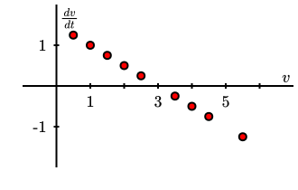
A graph of the points from parts (a) and (b) is shown in the following diagram:
described in detail following the image
A plot of points of the form \((v, \frac{dv}{dt})\) on the grid provided in part (a), using the data generated from the graphs in parts (a) and (b). The data points appear to lie on a line that passes through the point \((3,0)\) and has slope \(m = -0.5\text{.}\)
7.1.3.d
Answer.
The rate of change of velocity with respect to time is a linear function of velocity.

7.1.4 Solving a differential equation


7.2 Qualitative behavior of solutions to differential equations
7.2.2 Slope fields


Activity 7.2.2.
7.2.2.a
Answer.
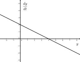
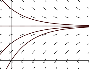
When \(y \lt 4\text{,}\) \(y\) is an increasing function of \(t\text{.}\) When \(y \gt 4\text{,}\) \(y\) is a decreasing function of \(t\text{.}\)
described in detail following the image
Plot of \(\frac{dy}{dt}\) as a function of \(y\text{.}\) The graph is a straight line with slope \(m=-\frac{1}{2}\) that passes through the point \((4,0)\text{.}\)
7.2.2.b
Answer.
described in detail following the image
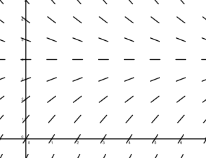
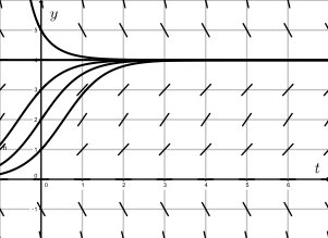
The slope field shows a constant solution of \(y = 4\) and that solutions that satisfy \(y(0) \gt 4\) are decreasing while solutions that satisfy \(y(0) \lt 4\) are increasing
.
For a fixed value of \(y\text{,}\) the line segments in the slope field all have the same slope, regardless of \(t\text{.}\) When \(y=4\text{,}\) the slopes are all \(0\text{.}\) When \(y \gt 4\text{,}\) the slopes are all negative, and the larger the value of \(y\) the more negative the slope is. When \(y \lt 4\text{,}\) the slopes are all positive, and the smaller the value of \(y\) the more positive the slope is.
7.2.2.c
Answer.
described in detail following the image
The graph shows the plots of four different solutions to the differential equation with the graphs superimposed on the slope field.
The solution that satisfies \(y(0) = 6\) is a decreasing, concave up function that approaches \(y = 4\) as \(t\) increases without bound. The solution that satisfies \(y(0) = 4\) is constant (that is, a horizontal line). The solutions that satisfy \(y(0) = 0\) and \(y(0) = 2\) are increasing, concave down functions that approach \(y = 4\) as \(t\) increases without bound.
7.2.2.d
Answer.
\begin{equation*} \frac{dy}{dt} = 2 \left( -\frac{1}{2} e^{-t/2} \right) = -e^{-t/2} \end{equation*}
and
\begin{equation*} -\frac{1}{2}( y - 4 ) = -\frac{1}{2} \left( 4 + 2e^{-t/2} \right) = -e^{-t/2} \end{equation*}
In addition, \(y(0) = 4 + 2e^0 = 6\text{.}\)

7.2.3 Equilibrium solutions and stability


Activity 7.2.3.
7.2.3.a
Answer.
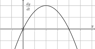
When \(y \lt 0\) and when \(y \gt 4\text{,}\) \(y\) is a decreasing function of \(t\text{.}\) When \(0 \lt y \lt 4\text{,}\) \(y\) is a increasing function of \(t\text{.}\)
described in detail following the image
Plot of \(\frac{dy}{dt}\) as a function of \(y\text{.}\) The graph is a concave down parabola that has zeros at \(y = 0\) and \(y=4\) with a maximum at the point \((2,2)\text{.}\)
7.2.3.c
Answer.
described in detail following the image
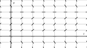
The slope field shows constant solutions of \(y = 0\) and \(y = 4\text{.}\) Solutions that satisfy \(y(0) \gt 4\) or \(y(0) \lt 0\) are decreasing, while solutions that satisfy \(0 \lt y(0) \lt 4\) are increasing
.
For a fixed value of \(y\text{,}\) the line segments in the slope field all have the same slope, regardless of \(t\text{.}\) When \(y \gt 4\text{,}\) the slopes are all negative, and the larger the value of \(y\) the more negative the slope is. When \(y=4\text{,}\) the slopes are all \(0\text{.}\) When \(0 \lt y \lt 4\text{,}\) the slopes are all positive, and the closer \(y\) is to \(0\) or \(4\) the closer the slope is to \(0\text{;}\) the largest positive slope occurs when \(y=2\text{.}\) Finally, when \(y \lt 0\text{,}\) the slopes are all negative, and the more negative the value of \(y\) the more negative the slope is.
7.2.3.d
Answer.
described in detail following the image
The graph shows the plots of the different solutions to the differential equation with the graphs superimposed on the slope field.
The solution that satisfies \(y(0) = 5\) is a decreasing, concave up function that approaches \(y = 4\) as \(t\) increases without bound. The solution that satisfies \(y(0) = 4\) is constant (that is, a horizontal line). The solutions that satisfy \(y(0) = 1\text{,}\) \(y(0) = 2\text{,}\) and \(y(0) = 3\) are increasing functions that approach \(y = 4\) as \(t\) increases without bound. Each of these three functions is concave down for all values of \(y\) such that \(y \gt 2\text{.}\) The solution that satisfies \(y(0) = 0\) is constant (that is, a horizontal line). Finally, the solution that satisfies \(y(0) = -1\)is a decreasing concave down function that decreases without bound.
7.2.3.g
Answer.
The left image is for an ustable equilibrium; the right image is for a stable equilibrium.

7.3 Euler’s method
7.3.2 Euler’s Method


Activity 7.3.2.
7.3.2.a
Answer.
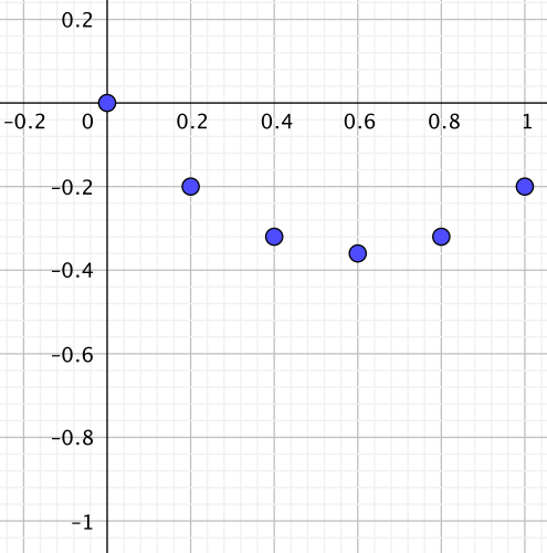
\(t_i\) \(y_i\) \(dy/dt\) \(\Delta y\)
\(0\) \(0\) \(-1\) \(-0.2\)
\(0.2\) \(-0.2\) \(-0.6\) \(-0.12\)
\(0.4\) \(-0.32\) \(-0.2\) \(-0.04\)
\(0.6\) \(-0.36\) \(0.2\) \(0.04\)
\(0.8\) \(-0.32\) \(0.6\) \(0.12\)
\(1.0\) \(-0.2\) \(1\) \(0.2\)
described in detail following the image
This image is a plot of the \(5\) points that result from applying Euler’s method to the given differential equation and the initial condition.
After the initial point \((0,0)\text{,}\) the plotted points are \((0.2,-0.2)\text{,}\) \((0.4,-0.32)\text{,}\) \((0.6,-0.36)\text{,}\) \((0.8,-0.32)\text{,}\) \((1,-0.2)\text{.}\)
7.3.2.b
Answer.
\(y = t^2 - t\text{,}\) with errors \(e_1 = 0.04\text{,}\) \(e_2 = 0.08\text{,}\) \(e_3 = 0.12\text{,}\) \(e_4 = 0.16\text{,}\) \(e_5 = 0.2\text{.}\)
7.3.2.d
Answer.
If we first think about how \(y_1\) is generated for the initial value problem \(\frac{dy}{dt} = f(t) = 2t-1, \ y(0) = 0\text{,}\) we see that \(y_1 = y_0 + \Delta t \cdot f(t_0)\text{.}\) Since \(y_0 = 0\text{,}\) we have \(y_1 = \Delta t \cdot f(t_0)\text{.}\) From there, we know that \(y_2\) is given by \(y_2 = y_1 + \Delta t f(t_1)\text{.}\) Substituting our earlier result for \(y_1\text{,}\) we see that \(y_2 = \Delta t \cdot f(t_0) + \Delta t f(t_1)\text{.}\) Continuing this process up to \(y_5\text{,}\) we get
\begin{equation*} y_5 = \Delta t \cdot f(t_0) + \Delta t f(t_1) + \Delta t f(t_2) + \Delta t f(t_3) + \Delta t f(t_4) \end{equation*}
This is precisely the left Riemann sum with five subintervals for the definite integral \(\int_0^1 (2t-1)~dt\text{.}\)


Activity 7.3.3.
7.3.3.a
Answer.
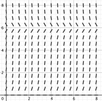
described in detail following the image
The slope field shows constant solutions of \(y = 0\) and \(y = 6\text{.}\) Solutions that satisfy \(y(0) \gt 6\) are decreasing, while solutions that satisfy \(0 \lt y(0) \lt 6\) are increasing
.
For a fixed value of \(y\text{,}\) the line segments in the slope field all have the same slope, regardless of \(t\text{.}\) When \(y \gt 6\text{,}\) the slopes are all negative, and the larger the value of \(y\) the more negative the slope is. When \(y=6\text{,}\) the slopes are all \(0\text{.}\) When \(0 \lt y \lt 6\text{,}\) the slopes are all positive, and the closer \(y\) is to \(0\) or \(6\) the closer the slope is to \(0\text{;}\) the largest positive slope occurs when \(y=3\text{.}\) Finally, when \(y = 0\text{,}\) the slopes are all zero.
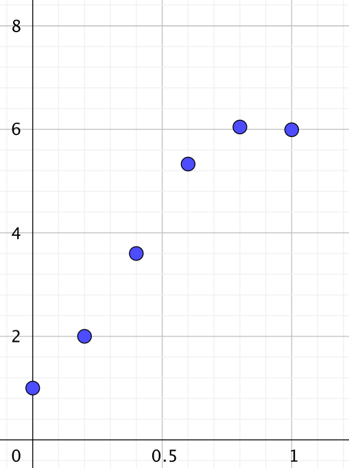
7.3.3.d
Answer.
\(t_i\) \(y_i\) \(dy/dt\) \(\Delta y\)
\(0.0\) \(1.0000\) \(5.0000\) \(1.0000\)
\(0.2\) \(2.0000\) \(8.0000\) \(1.6000\)
\(0.4\) \(3.6000\) \(8.6400\) \(1.7280\)
\(0.6\) \(5.3280\) \(3.5804\) \(0.7161\)
\(0.8\) \(6.0441\) \(-0.2664\) \(-0.0533\)
\(1.0\) \(5.9908\) \(0.0551\) \(0.0110\)
described in detail following the image
This image is a plot of the \(5\) points that result from applying Euler’s method to the given differential equation and the initial condition.
After the initial point \((0,1)\text{,}\) the plotted points are \((0.2,2)\text{,}\) \((0.4,3.6)\text{,}\) \((0.6,5.328)\text{,}\) \((0.8,6.0441)\text{,}\) \((1,5.9908)\text{.}\)

7.4 Separable differential equations
7.4.2 Solving separable differential equations


7.5 Modeling with differential equations
7.5.2 Developing a differential equation


Activity 7.5.3.

7.6 Population growth and the logistic equation
7.6.2 The earth’s population


Activity 7.6.2.
7.6.2.f
Answer.
\(t = \frac{1}{0.012041} \ln \left( \frac{12}{6.084}\right) \approx 56.41\text{,}\) or in the year 2056.

7.6.3 Solving the logistic differential equation


Activity 7.6.3.
7.6.3.d
Answer.
\(t = \frac{1}{-0.025} \ln \left( \frac{\left( \frac{12.5}{9} - 1 \right)}{1.0546}\right) \approx 39.9049\) (so in about year \(2040\)).

8 Taylor Polynomials and Taylor Series
8.1 Extending local linearization
8.1.2 Finding a quadratic approximation


Activity 8.1.2.
8.1.2.c
Answer.
Table 8.1.1. Formulas and values for \(f(x)\) and \(T_2(x)\text{.}\)
\(f(x)=\) \(e^x\) \(T_2(x)=\) \(b_0 + b_1 x + b_2 x^2\)
\(f'(x)=\) \(e^x\) \(T_2'(x)=\) \(b_1 + 2b_2 x\)
\(f''(x)=\) \(e^x\) \(T_2''(x)=\) \(2b_2\)
\(f(0)=\) \(1\) \(T_2(0)=\) \(b_0\)
\(f'(0)=\) \(1\) \(T_2'(0)=\) \(b_1\)
\(f''(0)=\) \(1\) \(T_2''(0)=\) \(2b_2\)
8.1.2.e
Answer.
\(b_0 = 1\text{;}\) \(b_1 = 1\text{;}\) \(b_2 = \frac{1}{2}\text{.}\) So, \(T_2(x) = 1 + x + \frac{1}{2} x^2\text{.}\)
8.1.2.f
Answer.
\(T_2(x)\) is a better approximation to \(f(x) = e^x\) near \(a = 0\) than the tangent line; \(|f(x)-T_2(x)| \lt 0.1\) for approximately \(-0.9 \lt x \lt 0.8\text{,}\) and for any \(x\)-value in that interval, \(|f(x)-T_2(x)| \lt |f(x)-T_1(x)|\text{.}\)

8.1.3 Over and over again


Activity 8.1.3.
8.1.3.a
Answer.
Table 8.1.5. Formulas and values for \(f(x)\) and \(T_3(x)\text{.}\)
\(f(x)=\) \(e^x\) \(T_3(x)=\) \(c_0 + c_1 x + c_2 x^2 + c_3 x^3\)
\(f'(x)=\) \(e^x\) \(T_3'(x)=\) \(c_1 + 2 c_2 x + 3 c_3 x^2\)
\(f''(x)=\) \(e^x\) \(T_3''(x)=\) \(2 c_2 + 3 \cdot 2 c_3 x\)
\(f'''(x)=\) \(e^x\) \(T_3'''(x)=\) \(3 \cdot 2 c_3\)
\(f(0)=\) \(1\) \(T_3(0)=\) \(c_0\)
\(f'(0)=\) \(1\) \(T_3'(0)=\) \(c_1\)
\(f''(0)=\) \(1\) \(T_3''(0)=\) \(2c_2\)
\(f'''(0)=\) \(1\) \(T_3'''(0)=\) \(6c_3\)
8.1.3.b
Answer.
\(c_0 = 1\text{;}\) \(c_1 = 1\text{;}\) \(c_2 = \frac{1}{2}\text{;}\) \(c_3 = \frac{1}{6}\text{.}\)
8.1.3.c
Answer.
\(T_3(x)\) appears to be an even better approximation than \(T_2(x)\) near \(a = 0\) and that the quality of the approximation extends further; \(|f(x)-T_3(x)| \lt 0.1\) for approximately \(-1.3 \lt x \lt 1.1\text{.}\)
8.1.3.d
Answer.
\(T_4(x) = 1 + x + \frac{1}{2}x^2 + \frac{1}{6} x^3 + \frac{1}{24}x^4\text{;}\) \(T_4(x)\) is an even better approximation to \(f(x) = e^x\) and on a still wider interval.

8.1.4 As the degree of the approximation increases


Activity 8.1.4.
8.1.4.a
Answer.
The first seven columns and eleven rows of the spreadsheet are:
Table 8.1.11. Comparing \(f(x) = e^x\) and its degree \(1\text{,}\) \(2\text{,}\) \(3\text{,}\) \(4\) and approximations near \(a = 0\text{.}\)
\(\Delta x\) \(x\) \(f(x)\) \(T_1(x)\) \(T_2(x)\) \(T_3(x)\) \(T_4(x)\)
\(0.1\) \(-1.0\) \(0.36787\) \(0.00000\) \(0.50000\) \(0.33333\) \(0.37500\)
\(0.1\) \(-0.9\) \(0.40657\) \(0.10000\) \(0.50500\) \(0.38350\) \(0.41083\)
\(0.1\) \(-0.8\) \(0.44933\) \(0.20000\) \(0.52000\) \(0.43467\) \(0.45173\)
\(0.1\) \(-0.7\) \(0.49659\) \(0.30000\) \(0.54500\) \(0.48783\) \(0.49784\)
\(0.1\) \(-0.6\) \(0.54881\) \(0.40000\) \(0.58000\) \(0.54400\) \(0.54940\)
\(0.1\) \(-0.5\) \(0.60653\) \(0.50000\) \(0.62500\) \(0.60417\) \(0.60677\)
\(0.1\) \(-0.4\) \(0.67032\) \(0.60000\) \(0.68000\) \(0.66933\) \(0.67040\)
\(0.1\) \(-0.3\) \(0.74082 \) \(0.70000 \) \(0.74500 \) \(0.74050 \) \(0.74084\)
\(0.1\) \(-0.2\) \(0.81873 \) \(0.80000 \) \(0.82000 \) \(0.81867 \) \(0.81873\)
\(0.1\) \(-0.1\) \(0.90484 \) \(0.90000 \) \(0.90500 \) \(0.90483 \) \(0.90484\)
\(0.1\) \(0.0\) \(1.00000\) \(1.00000\) \(1.00000\) \(1.00000\) \(1.00000\)
The next four columns and four rows of the spreadsheet are:
Table 8.1.12. The absolute error between \(f(x) = e^x\) and its degree \(1\text{,}\) \(2\text{,}\) \(3\text{,}\) and \(4\) approximations at \(x=-1\) and \(x=-0.9\text{.}\)
\(|f(x)-T_1(x)|\) \(|f(x)-T_2(x)|\) \(|f(x)-T_3(x)|\) \(|f(x)-T_4(x)|\)
\(0.36787\) \(0.13212\) \(0.03454\) \(0.00712\)
\(0.30657\) \(0.09843\) \(0.02307\) \(0.00426\)
\(0.24933 \) \(0.07067 \) \(0.01466 \) \(0.00240\)
\(0.19659 \) \(0.04841 \) \(0.00875 \) \(0.00125\)
8.1.4.b
Answer.
\(|f(-1) - T_2(-1)| \approx 0.13212\text{;}\) \(|f(1) - T_2(1)| \approx 0.21828\text{.}\)
8.1.4.c
Answer.
\(|f(-1) - T_3(-1)| \approx 0.03455\text{;}\) \(|f(1) - T_3(1)| \approx 0.05162\text{.}\)
8.1.4.d
Answer.
\(|f(-1) - T_4(-1)| \approx 0.00712\text{;}\) \(|f(1) - T_4(1)| \approx 0.00995\text{.}\)
8.1.4.e
Answer.
As the degree of the approximation increases, at each fixed \(x\)-value, the approximation gets better, and in addition the interval of values on which the approximation is within a certain tolerance gets wider.
8.1.4.f
Answer.
Answers will vary. But, as we widen the interval of \(x\)-values, the errors of each polynomial approximation increase near the endpoints of the interval.

8.2 Taylor polynomials
8.2.2 Taylor polynomials


Activity 8.2.2.
8.2.2.a
Answer.
Table 8.2.7. Finding the derivatives of \(f(x) = \cos(x)\) at \(a = 0\text{.}\)
\(f(x) =\) \(\cos(x)\) \(f(0) =\) \(\cos(0) = 1\)
\(f'(x) = \) \(-\sin(x)\) \(f'(0) = \) \(0\)
\(f''(x) = \) \(-\cos(x)\) \(f''(0) = \) \(-1\)
\(f'''(x) = \) \(\sin(x)\) \(f'''(0) = \) \(0\)
\(f^{(4)}(x) = \) \(\cos(x)\) \(f^{(4)}(0) = \) \(1\)
\(f^{(5)}(x) = \) \(-\sin(x)\) \(f^{(5)}(0) = \) \(0\)
\(f^{(6)}(x) = \) \(-\cos(x)\) \(f^{(6)}(0) = \) \(-1\)
\(f^{(7)}(x) = \) \(\sin(x)\) \(f^{(7)}(0) = \) \(0\)
\(f^{(8)}(x) = \) \(\cos(x)\) \(f^{(8)}(0) = \) \(1\)
8.2.2.b
Answer.
\begin{align*} T_2(x) \amp= 1 + 0x - \frac{1}{2!}x^2 \\ T_4(x) \amp= 1 + 0x - \frac{1}{2!}x^2 + 0x^3 + \frac{1}{4!}x^4 \\ T_6(x) \amp= 1 + 0x - \frac{1}{2!}x^2 + 0x^3 + \frac{1}{4!}x^4 + 0x^5 - \frac{1}{6!}x^6\\ T_8(x) \amp= 1 + 0x - \frac{1}{2!}x^2 + 0x^3 + \frac{1}{4!}x^4 + 0x^5 - \frac{1}{6!}x^6 + 0x^7 + \frac{1}{8!}x^8 \end{align*}
8.2.2.c
Answer.
\(T_{10}(x) = 1 - \frac{1}{2!}x^2 + \frac{1}{4!}x^4 - \frac{1}{6!}x^6 + \frac{1}{8!}x^8 - \frac{1}{10!}x^{10}\text{.}\)
8.2.2.d
Answer.
described in detail following the image
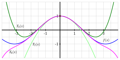
The function \(f(x)=\cos(x)\) graphed together with its degree \(2\text{,}\) \(4\text{,}\) and \(6\) Taylor polynomial approximations near the point \((0,f(0))\text{.}\)
The graph shows that the function and the three Taylor approximations all intersect at the point \((0,f(0))\text{,}\) have the same slope at that point, and look like they have the same curvature at that point.
The four functions are very close together on the interval \((-1,1)\text{,}\) but outside of that interval there start to be visual differences as the parabola continues to open downward, but the function \(\cos(x)\) oscillates and the degree \(4\) and \(6\) approximations follow the function for longer.
The degree \(4\) Taylor polynomial approximation looks very close to the function \(\cos(x)\) on the interval \((-1.75,1.75)\text{,}\) and the degree \(6\) Taylor polynomial approximation looks very close to the function \(\cos(x)\) on the interval \((-2.5,2.5)\text{.}\)
Figure 8.2.10. The function \(f(x)=\cos(x)\) and its degree \(2\text{,}\) \(4\text{,}\) and \(6\) Taylor polynomial approximations near the point \((0,f(0))\text{.}\)
As the degree of the approximation increases, the accuracy of the approximation improves at each fixed \(x\)-value and in how large the interval is on which the approximation is accurate.
8.2.2.e
Answer.
Table 8.2.14. Comparing \(f(x) = \cos(x)\) and its degree \(2\text{,}\) \(4\text{,}\) and \(6\) approximations near \(a = 0\text{.}\)
\(\Delta x\) \(x\) \(f(x)\) \(T_2(x)\) \(T_4(x)\) \(T_6(x)\)
\(0.2\) \(-2.0\) \(-0.41615\) \(-1.00000\) \(-0.33333\) \(-0.42222\)
\(0.2\) \(-1.8\) \(-0.22720\) \(-0.62000\) \(-0.18260\) \(-0.22984\)
\(0.2\) \(-1.6\) \(-0.02920\) \(-0.28000\) \(-0.00693\) \(-0.03024\)
\(\cdots\) \(\cdots\) \(\cdots\) \(\cdots\) \(\cdots\) \(\cdots\)
\(0.2\) \(1.6\) \(-0.02920\) \(-0.28000\) \(-0.00693\) \(-0.03024\)
\(0.2\) \(1.8\) \(-0.22720\) \(-0.62000\) \(-0.18260\) \(-0.22984\)
\(0.2\) \(2.0\) \(-0.41615\) \(-1.00000\) \(-0.33333\) \(-0.42222\)
Table 8.2.15. The absolute error between \(f(x) = \cos(x)\) and its degree \(2\text{,}\) \(4\text{,}\) and \(6\) approximations.
\(|f(x)-T_2(x)|\) \(|f(x)-T_4(x)|\) \(|f(x)-T_6(x)|\)
\(0.58385\) \(0.08281\) \(0.00608\)
\(0.39280\) \(0.04460\) \(0.00263\)
\(0.25080\) \(0.02227\) \(0.00104\)
\(\cdots\) \(\cdots\) \(\cdots\)
\(0.25080\) \(0.02227\) \(0.00104\)
\(0.39280\) \(0.04460\) \(0.00263\)
\(0.58385\) \(0.08281\) \(0.00608\)
\(|f(x) - T_2(x)| \lt 0.1\) for roughly \(-1.2 \lt x \lt 1.2\text{;}\) \(|f(x) - T_4(x)| \lt 0.1\) for \(-2 \lt x \lt 2\text{;}\) \(|f(x) - T_6(x)| \lt 0.1\) for approximately \(-2.8 \lt x \lt 2.8\text{.}\)

8.2.3 Taylor polynomial approximations centered at an arbitrary value \(a\)


Activity 8.2.3.
8.2.3.a
Answer.
\(f(x) =\) \(\ln(x)\) \(f(1) =\) \(0\)
\(f'(x) = \) \(x^{-1}\) \(f'(1) = \) \(1\)
\(f''(x) = \) \(-1 \cdot x^{-2}\) \(f''(1) = \) \(-1\)
\(f'''(x) = \) \((-2)(-1)x^{-3}\) \(f'''(1) = \) \((-2)(-1)\)
\(f^{(4)}(x) = \) \((-3)(-2)(-1)x^{-4}\) \(f^{(4)}(1) = \) \((-3)(-2)(-1)\)
8.2.3.b
Answer.
\(T_4(x) = 1 (x-1) - \frac{1}{2} (x-1)^2 + \frac{1}{3}(x-1)^3 - \frac{1}{4}(x-1)^4 \text{.}\)
8.2.3.c
Answer.
described in detail following the image
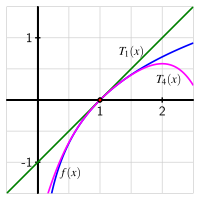
The function \(f(x)=\ln(x)\) graphed together with its degree \(1\) and \(4\) Taylor polynomial approximations near the point \((1,f(1))\text{.}\)
The graph shows that the function and the two Taylor approximations all intersect at the point \((1,f(1))\) and have the same slope at that point.
The three functions are very close together on the interval \((0.5,1.5)\text{,}\) but outside of that interval there start to be visual differences as the tangent line continues straight, but the function \(\ln(x)\) is curved, and the degree \(4\) approximation stays close to the function for longer.
The degree \(4\) Taylor polynomial approximation looks very close to the function \(\ln(x)\) on the interval \((0.3,1.75)\text{.}\)
\(T_4(x)\) provides a much more accurate approximation of \(f(x)\) than \(T_1(x)\text{.}\)
8.2.3.e
Answer.
\(T_5(x) = 1 (x-1) - \frac{1}{2} (x-1)^2 + \frac{1}{3}(x-1)^3 - \frac{1}{4}(x-1)^4 + \frac{1}{5}(x-1)^5\text{;}\) \(T_6(x) = 1 (x-1) - \frac{1}{2} (x-1)^2 + \frac{1}{3}(x-1)^3 - \frac{1}{4}(x-1)^4 + \frac{1}{5}(x-1)^5 - \frac{1}{6}(x-1)^6\text{.}\)
\(|f(x) - T_5(x)| \lt 0.1\) for about \(0.24 \lt x \lt 1.999\text{;}\) \(|f(x) - T_6(x)| \lt 0.1\) for about \(0.21 \lt x \lt 2\text{.}\) While the interval of accuracy gets wider as the degree increases, it seems not to extend past \(x = 2\) and doesn’t move much to the left.


Activity 8.2.4.
8.2.4.a
Answer.
\(f(x) =\) \(\ln(x)\) \(f(2) =\) \(\ln(2)\)
\(f'(x) = \) \(x^{-1}\) \(f'(2) = \) \(\frac{1}{2}\)
\(f''(x) = \) \(-1 \cdot x^{-2}\) \(f''(2) = \) \(-\frac{1}{2^2}\)
\(f'''(x) = \) \((-2)(-1)x^{-3}\) \(f'''(2) = \) \(\frac{(-2)(-1)}{2^3}\)
\(f^{(4)}(x) = \) \((-3)(-2)(-1)x^{-4}\) \(f^{(4)}(2) = \) \(\frac{(-3)(-2)(-1)}{2^4}\)
8.2.4.b
Answer.
\(T_4(x) = \ln(2) + \frac{1}{2}(x-2) - \frac{1}{2 \cdot 2^2} (x-2)^2 + \frac{1}{3 \cdot 2^3}(x-2)^3 - \frac{1}{4 \cdot 2^4}(x-2)^4\text{.}\)
8.2.4.c
Answer.
described in detail following the image
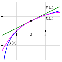
The function \(f(x)=\ln(x)\) graphed together with its degree \(1\) and \(4\) Taylor polynomial approximations near the point \((2,f(2))\text{.}\)
The graph shows that the function and the two Taylor approximations all intersect at the point \((2,f(2))\) and have the same slope at that point.
The three functions are very close together on the interval \((1.5,2.5)\text{,}\) but outside of that interval there start to be visual differences as the tangent line continues straight, but the function \(\ln(x)\) is curved, and the degree \(4\) approximation stays close to the function for longer.
The degree \(4\) Taylor polynomial approximation looks very close to the function \(\ln(x)\) on the interval \((0.7,3.5)\text{.}\)
\(T_4(x)\) provides a much better approximation of \(f(x)\) near \(a = 2\) and on a wider interval.
8.2.4.e
Answer.
\(T_5(x) = \ln(2) + \frac{1}{2}(x-2) - \frac{1}{2 \cdot 2^2} (x-2)^2 + \frac{1}{3 \cdot 2^3}(x-2)^3 - \frac{1}{4 \cdot 2^4}(x-2)^4 + \frac{1}{5 \cdot 2^5} (x-2)^5 \text{;}\) \(T_6(x) = \ln(2) + \frac{1}{2}(x-2) - \frac{1}{2 \cdot 2^2} (x-2)^2 + \frac{1}{3 \cdot 2^3}(x-2)^3 - \frac{1}{4 \cdot 2^4}(x-2)^4 + \frac{1}{5 \cdot 2^5} (x-2)^5 - \frac{1}{6 \cdot 2^6} (x-2)^6 \text{.}\)
\(|f(x) - T_5(x)| \lt 0.1\) for roughly \(0.48 \lt x \lt 4\text{;}\) \(|f(x) - T_6(x)| \lt 0.1\) for about \(0.42 \lt x lt 4\text{.}\) By moving to \(a = 2\text{,}\) which is further away from the asymptote at \(x = 0\text{,}\) we can get approximations of \(ln(x)\) that seem to be good all the way up to \(x = 4\text{.}\)

8.3 Geometric sums
8.3.2 Finite Geometric Series


Activity 8.3.2.
8.3.2.a
Answer.
\(\frac{2}{5} \cdot S_n = \frac{2}{5} + \left(\frac{2}{5}\right)^2 + \left(\frac{2}{5}\right)^3 + \cdots + \left(\frac{2}{5}\right)^n \text{.}\)
8.3.2.b
Answer.
The key observation is that \(1 + \frac{2}{5} + \left(\frac{2}{5}\right)^2 + \cdots + \left(\frac{2}{5}\right)^{n-1} - \frac{2}{5} - \left(\frac{2}{5}\right)^2 - \left(\frac{2}{5}\right)^3 - \cdots - \left(\frac{2}{5}\right)^n = 1 - \left(\frac{2}{5}\right)^n\text{.}\)

8.3.3 Infinite Geometric Series


Activity 8.3.3.
8.3.3.a
Answer.
\(S_5 = \frac{a - ar^5}{1-r} = \frac{1 - (1/3)^5}{1-(1/3)} = \frac{121}{81} \approx 1.4938 \text{;}\) \(S_{10} = \frac{a - ar^{10}}{1-r} = \frac{1 - (1/3)^{10}}{1-(1/3)} = \frac{29524}{19683} \approx 1.49997 \text{;}\) \(S = \frac{a}{1-r} = \frac{1}{1-\frac{1}{3}} = \frac{1}{\frac{2}{3}} = \frac{3}{2} \text{.}\)
8.3.3.b
Answer.
\(S_5 = \frac{a - ar^5}{1-r} = \frac{4 - 4\cdot(-1/2)^5}{1-(-1/2)} = \frac{11}{4} \text{;}\) \(S_{10} = \frac{a - ar^{10}}{1-r} = \frac{4 - 4\cdot(-1/2)^{10}}{1-(-1/2)} = \frac{341}{128} = 2.6640625 \text{;}\) \(S = \frac{a}{1-r} = \frac{4}{1+\frac{1}{2}} = \frac{4}{\frac{3}{2}} = \frac{8}{3} \text{.}\)
8.3.3.c
Answer.
\(S_5 = \frac{a - ar^5}{1-r} = \frac{2 - 2\cdot(4/3)^5}{1-(4/3)} = \frac{1562}{81} \approx 19.284 \text{;}\) \(S_{10} = \frac{a - ar^{10}}{1-r} = \frac{2 - 2\cdot(4/3)^{10}}{1-(4/3)} = \frac{1979054}{19683} \approx 100.546 \text{;}\) the infinite series diverges.
8.3.3.d
Answer.
\(S_5 = \frac{a - ar^5}{1-r} = \frac{5 - 5\cdot(3/4)^5}{1-(3/4)} = \frac{3905}{256} \approx 15.254 \text{;}\) \(S_{10} = \frac{a - ar^{10}}{1-r} = \frac{5 - 5\cdot(3/4)^{10}}{1-(3/4)} = \frac{4947635}{262144} \approx 18.874 \text{;}\) \(S = \frac{a}{1-r} = \frac{5}{1-\frac{3}{4}} = 20 \text{.}\)
8.3.3.e
Answer.
\(S_5 = \frac{a - ar^5}{1-r} = \frac{\frac{4}{3} - \frac{4}{3} \cdot (-2/3)^5}{1-(-2/3)} = \frac{220}{243} \approx 0.905 \text{;}\) \(S_{10} = \frac{a - ar^{10}}{1-r} = \frac{\frac{4}{3} - \frac{4}{3} \cdot (-2/3)^{10}}{1-(-2/3)} = \frac{46420}{59049} \approx 0.786 \text{;}\) \(S = \frac{a}{1-r} = \frac{\frac{4}{3}}{1+\frac{2}{3}} = \frac{4}{5} = 0.8 \text{.}\)

8.3.4 How geometric series naturally connect to Taylor polynomials


Activity 8.3.4.
8.3.4.a
Answer.
\(f(x) =\) \(\frac{1}{1-x} = (1-x)^{-1}\)
\(f'(x) =\) \((-1)(1-x)^{-2}(-1)\)
\(f''(x) = \) \((-2)(-1)(1-x)^{-3}(-1)(-1)\)
\(f'''(x) = \) \((-3)(-2)(-1)(1-x)^{-4}(-1)(-1)(-1)\)
\(f^{(4)}(x) = \) \((-4)(-3)(-2)(-1)(1-x)^{-5}(-1)(-1)(-1)(-1)\)
\(f^{(5)}(x) = \) \((-5)(-4)(-3)(-2)(-1)(1-x)^{-6}(-1)(-1)(-1)(-1)(-1)\)
8.3.4.b
Answer.
\(f(0) =\) \(\frac{1}{1-0} = 1\) \(c_0 =\) \(f(0) = 1\)
\(f'(0) =\) \((-1)(1-0)^{-2}(-1) = 1\) \(c_1 =\) \(\frac{f'(0)}{1!} = \frac{1}{1!} = 1\)
\(f''(0) = \) \((-2)(-1)(1)^{-3}(-1)(-1) = 2!\) \(c_2 =\) \(\frac{f''(0)}{2!} = \frac{2!}{2!} = 1 \)
\(f'''(0) = \) \((-3)(-2)(-1)(1)^{-4}(-1)(-1)(-1) = 3!\) \(c_3 = \) \(\frac{f'''(0)}{3!} = \frac{3!}{3!} = 1 \)
\(f^{(4)}(0) = \) \((-4)(-3)(-2)(-1)(1)^{-5}(-1)(-1)(-1)(-1) = 4!\) \(c_4 =\) \(\frac{f^{(4)}(0)}{4!} = \frac{4!}{4!} = 1 \)
\(f^{(5)}(0) = \) \((-5)(-4)(-3)(-2)(-1)(1)^{-6}(-1)(-1)(-1)(-1)(-1) = 5!\) \(c_5 =\) \(\frac{f^{(5)}(0)}{5!} = \frac{5!}{5!} = 1 \)
8.3.4.c
Answer.
\(T_5(x) = 1 + x + x^2 + \cdots + x^5\) and \(T_n(x) = 1 + x + x^2 + \cdots + x^n \text{.}\)
8.3.4.e
Answer.
\(T(x) = 1 + x + x^2 + \cdots + x^n + \cdots\) which is an infinite geometric sum with \(a = 1\) and \(r = x\) whose sum (for \(|r| = |x| \lt 1\)) is \(\frac{a}{1-r} = \frac{1}{1-x} = f(x)\text{.}\)

8.4 Taylor series
8.4.2 Taylor series and the Ratio Test


Activity 8.4.2.
8.4.2.d
Answer.
On \(1 \lt x \lt 3\text{,}\) \(T_{10}\) and \(f\) are nearly indistinguishable for most of the interval. This suggests that \(T(x)\) is the Taylor series of \(f(x) = \ln(2) - \ln(3-x)\text{.}\)

8.4.3 Taylor series of several important functions


Activity 8.4.3.
8.4.3.a
Answer.
\(f^{(k)}(0) = 1\) for every natural number \(k\) because \(f^{(k)}(x) = e^x\) for every natural number \(k\text{.}\)
8.4.3.b
Answer.
\(T_f(x) = \sum_{n=0}^{\infty} \frac{1}{k!} x^k = 1 + x + \frac{1}{2!}x^2 + \frac{1}{3!}x^3 + \cdots + \frac{1}{n!}x^n + \cdots\)
8.4.3.d
Answer.
\(r(x) = \lim_{n \to \infty} r_n(x) = 0 \text{;}\) \(|r(x)| \lt 1\) for every value of \(x\text{;}\) \(T_f(x)\) converges for every real number \(x\text{.}\)
8.4.3.e
Answer.
\(f(x)\) and \(T_{10}(x)\) are almost indistinguishable on the interval \(-4 \lt x \lt 4\text{;}\) \(f(x)\) and \(T_{20}(x)\) are almost indistinguishable on \(-8 \lt x \lt 8\text{.}\)

8.5 Finding and using Taylor series
8.5.2 Using substitution and algebra to find new Taylor series expressions


Activity 8.5.2.
8.5.2.a
Answer.
\(g(x) = x^3 \sin(x^2) = x^5 - \frac{1}{3!}x^9 + \frac{1}{5!}x^{13} - \cdots \text{,}\) which converge for all real numbers \(x\text{.}\)
8.5.2.b
Answer.
\(h(x) = 1 - x^4 + \frac{1}{2!}x^8 - \frac{1}{3!}x^{12} + \cdots\text{,}\) which converges for all real numbers \(x\text{.}\)
8.5.2.c
Answer.
\(p(x) = 1 - 5x + (-5x)^2 + (-5x)^3 + \cdots = 1 - 5x + 5^2x^2 - 5^3x^3 + \cdots\text{,}\) which converges whenever \(|-5x| \lt 1\text{,}\) or for \(-\frac{1}{5} \lt x \lt \frac{1}{5}\text{.}\)
8.5.2.d
Answer.
\(q(x) = x^6 - \frac{1}{2}x^{10} + \frac{1}{3}x^{14} - \cdots\text{,}\) which converges for \(|x| \lt 1\text{.}\)
8.5.2.e
Answer.
\(r(x) = 1 + \frac{1}{2!}(3x) + \frac{1}{3!}(3x)^2 + \frac{1}{4!}(3x)^3 + \cdots\text{,}\) which converges for all real numbers \(x\text{.}\)

8.5.3 Differentiating and integrating Taylor series


Activity 8.5.3.
8.5.3.a
8.5.3.a.iii
Answer.
\(\frac{d}{dx}\left[ (-1)^{k} \frac{x^{2k}}{(2k)!} \right] = (-1)^{k} \frac{1}{(2k-1)!} \cdot x^{2k-1}\)


Activity 8.5.4.
8.5.4.b
Answer.
\(\int_0^x e^{-t^2} \, dt = x - \frac{1}{3}x^3 + \frac{1}{5 \cdot 2!}x^5 - \frac{1}{7 \cdot 3!} x^7 + \cdots \)
8.5.4.c
Answer.
\(\erf(x) = \frac{2}{\sqrt{\pi}} \left( x - \frac{1}{3}x^3 + \frac{1}{5 \cdot 2!}x^5 - \frac{1}{7 \cdot 3!} x^7 + \cdots \right)\)
8.5.4.e
Answer.
\(\erf(0.5) \approx \frac{2}{\sqrt{\pi}} \left( \frac{1}{2} - \frac{1}{3 \cdot 2^3} + \frac{1}{5 \cdot 2! \cdot 2^5} - \frac{1}{7 \cdot 3! \cdot 2^7}\right) = 0.52049 \ldots\)

8.6 Quantifying the accuracy of approximations
8.6.2 Alternating series of real numbers


Activity 8.6.2.
8.6.2.a
Answer.
\(\sin(1) \approx 1 - \frac{1}{3!} + \frac{1}{5!} - \frac{1}{7!} = \frac{4241}{5040} = 0.8414682539682539\ldots \text{,}\) and this approximation has error at most \(\frac{1}{9!} \approx 0.00000276\text{.}\)
8.6.2.b
Answer.
\(\int_0^1 e^{-x^2} \, dx \approx 1 - \frac{1}{3} + \frac{1}{2! \cdot 5} - \frac{1}{3! \cdot 7} + \frac{1}{4! \cdot 9} - \frac{1}{5! \cdot 11} + \frac{1}{6! \cdot 13} = \frac{1614779}{2162160} = 0.7468360343\ldots\) and this approximation has error at most \(\frac{1}{7! \cdot 15} = \frac{1}{756600} \approx 0.0000132\)
8.6.2.c
Answer.
\(\int_0^1 \cos(x^2) \, dx \approx 1 - \frac{1}{5 \cdot 2!} + \frac{1}{9 \cdot 4!} - \frac{1}{13 \cdot 6!} = \frac{25399}{28080} = 0.904522792022792022792\ldots \) and this approximation has error at most \(\frac{1}{17 \cdot 8!} = \frac{1}{685440} = 0.0000014589 \ldots \text{.}\)
8.6.2.d
Answer.
The alternating series
\begin{equation*} 1 - \frac{1}{2} \cdot 1^2 + \frac{1}{3} \cdot 1^3 - \cdots + (-1)^{n-1} \frac{1}{n} \cdot 1^n + \cdots \end{equation*}
converges by the Alternating Series Theorem, and its exact sum is \(\ln(2)\text{.}\)
Using the Alternating Series Estimation Theorem to approximate within \(0.01\) results in
\begin{equation*} \ln(2) \approx 1 - \frac{1}{2} + \frac{1}{3} - \cdots + \frac{1}{99} = 0.69817217931 \ldots\text{.} \end{equation*}

8.6.3 Error Approximations for Taylor Polynomials


Activity 8.6.3.
8.6.3.a
Answer.
For \(f(x) = e^2\text{,}\) the Lagrange Error Bound gives \(\left| f(2) - T_{10}(2) \right| \leq e^2 \cdot \frac{|2-0|^{11}}{(11)!} = \frac{e^2 \cdot 2^{11}}{(11)!} \approx 0.00037910821 \text{.}\) The actual error is \(\left| f(2) - T_{10}(2) \right| \approx 0.00006138994 \)
8.6.3.b
Answer.
Using \(M = 1\) as the bound on the \((n+1)^{\text{st}}\) derivative of \(\cos(x)\text{,}\) the Lagrange error bound tells us that we need to use \(n = 11\) (\(n+1 = 12\)) to achieve the desired accuracy, and that \(\cos(1) \approx T_{10}(1) = 1 - \frac{1^2}{2!} + \frac{1^4}{4!} - \cdots - \frac{1^{10}}{10!} \approx 0.54030230379189\text{.}\)