What does it mean to say that a function is concave up or concave down? How are these characteristics connected to certain properties of the derivative of the function?
Given a differentiable function \(y= f(x)\text{,}\) we know that its derivative, \(y = f'(x)\text{,}\) is a related function whose output at \(x=a\) tells us the slope of the tangent line to \(y = f(x)\) at the point \((a,f(a))\text{.}\) That is, heights on the derivative graph tell us the values of slopes on the original function’s graph.
At a point where \(f'(x)\) is positive, the slope of the tangent line to \(f\) is positive. Therefore, on an interval where \(f'(x)\) is positive, the function \(f\) is increasing (or rising). Similarly, if \(f'(x)\) is negative on an interval, the graph of \(f\) is decreasing (or falling).
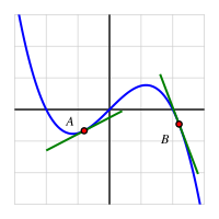
The derivative of \(f\) tells us not only whether the function \(f\) is increasing or decreasing on an interval, but also how the function \(f\) is increasing or decreasing. Look at the two tangent lines shown in Figure 1.6.1. We see that near point \(A\) the value of \(f'(x)\) is positive and relatively close to zero, so near that point the graph is rising slowly. By contrast, near point \(B\text{,}\) the derivative is negative and relatively large in absolute value, so \(f\) is decreasing rapidly near \(B\text{.}\)
Besides asking whether the value of the derivative function is positive or negative and whether it is large or small, we can also ask “how is the derivative changing?”
Because the derivative, \(y = f'(x)\text{,}\) is itself a function, we can consider taking its derivative — the derivative of the derivative — and ask “what does the derivative of the derivative tell us about how the original function behaves?” We start with an investigation of a moving object.
Given a function \(f(x)\) defined on the interval \((a,b)\text{,}\) we say that \(f\) is increasing on \((a,b)\) provided that for all \(x_1\text{,}\)\(x_2\) in the interval \((a,b)\text{,}\) if \(x_1 \lt x_2\text{,}\) then \(f(x_1) \lt f(x_2)\text{.}\) Similarly, we say that \(f\) is decreasing on \((a,b)\) provided that for all \(x_1\text{,}\)\(x_2\) in the interval \((a,b)\text{,}\) if \(x_1 \lt x_2\text{,}\) then \(f(x_1) \gt f(x_2)\text{.}\)
Simply put, an increasing function is one that is rising as we move from left to right along the graph, and a decreasing function is one that falls as the value of the input increases. If the function has a derivative, the sign of the derivative tells us whether the function is increasing or decreasing.
Let \(f\) be a function that is differentiable on an interval \((a,b)\text{.}\) It is possible to show that if \(f'(x) > 0\) for every \(x\) such that \(a \lt x \lt b\text{,}\) then \(f\) is increasing on \((a,b)\text{;}\) similarly, if \(f'(x) \lt 0\) on \((a,b)\text{,}\) then \(f\) is decreasing on \((a,b)\text{.}\)
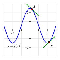
A function that is decreasing on the intervals \(-3 \lt x \lt -2\) and \(0 \lt x \lt 2\) and increasing on \(-2 \lt x \lt 0\) and \(2 \lt x \lt 3\text{.}\)
Figure1.6.3.A function that is decreasing on the intervals \(-3 \lt x \lt -2\) and \(0 \lt x \lt 2\) and increasing on \(-2 \lt x \lt 0\) and \(2 \lt x \lt 3\text{.}\)
For example, the function pictured in Figure 1.6.3 is increasing on the entire interval \(-2 \lt x \lt 0\text{,}\) and decreasing on the interval \(0 \lt x \lt 2\text{.}\) Note that the value \(x = 0\) is not included in either interval since at this location, the function is changing from increasing to decreasing.
We are now accustomed to investigating the behavior of a function by examining its derivative. The derivative of a function \(f\) is a new function given by the rule
Because \(f'\) is itself a function, it is perfectly feasible for us to consider the derivative of the derivative, which is the new function \(y = [f'(x)]'\text{.}\) We call this resulting function the second derivative of \(y = f(x)\text{,}\) and denote the second derivative by \(y = f''(x)\text{.}\) Consequently, we will sometimes call \(f'\) “the first derivative” of \(f\text{,}\) rather than simply “the derivative” of \(f\text{.}\)
Let \(f\) be a function and \(x\) an input value in the function’s domain. We define the second derivative of \(f\), a new function called \(f''(x)\text{,}\) by the formula
The meaning of the derivative function still holds, so when we compute \(y = f''(x)\text{,}\) this new function measures slopes of tangent lines to the curve \(y = f'(x)\text{,}\) as well as the instantaneous rate of change of \(y = f'(x)\text{.}\) In other words, just as the first derivative measures the rate at which the original function changes, the second derivative measures the rate at which the first derivative changes. The second derivative will help us understand how the rate of change of the original function is itself changing.
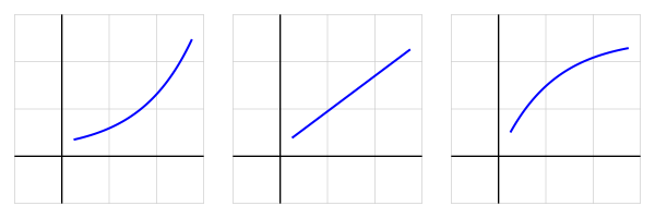
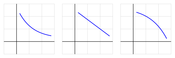
In addition to asking whether a function is increasing or decreasing, it is also natural to inquire how a function is increasing or decreasing. There are three basic behaviors that an increasing function can demonstrate on an interval, as pictured in Figure 1.6.5: the function can increase more and more rapidly, it can increase at the same rate, or it can increase in a way that is slowing down. Fundamentally, we are beginning to think about how a particular curve bends, with the natural comparison being made to lines, which don’t bend at all. More than this, we want to understand how the bend in a function’s graph is tied to behavior characterized by the first derivative of the function.
On the leftmost curve in Figure 1.6.5, imagine drawing a sequence of tangent lines to the curve. As we move from left to right, the slopes of those tangent lines will increase. Therefore, the rate of change of the pictured function is increasing, and this explains why we sometimes say this function is increasing at an increasing rate. For the rightmost graph in Figure 1.6.5, observe that as \(x\) increases, the function increases, but the slopes of the tangent lines decrease. This function is increasing at a decreasing rate.
Similar options hold for how a function can decrease. Here we must be extra careful with our language, because decreasing functions involve negative slopes. Negative numbers present an interesting tension between common language and mathematical language. For example, it can be tempting to say that “\(-100\) is bigger than \(-2\text{.}\)” But we must remember that “greater than” describes how numbers lie on a number line: \(x \gt y\) provided that \(x\) lies to the right of \(y\text{.}\) So of course, \(-100\) is less than \(-2\text{.}\) Informally, it can be helpful to say that “\(-100\) is more negative than \(-2\text{.}\)” When a function’s values are negative, and those values get more negative as the input increases, the function must be decreasing. The situation gets a bit more complicated when we think about how the slope of the tangent line to a decreasing function changes as we move from left to right.
The three graphs shown in Figure 1.6.6 show three possibilities for how a function can decrease in a consistent way. The middle graph depicts a function decreasing at a constant rate. If we imagine a sequence of tangent lines on the leftmost graph, the slopes of the tangent lines get less and less negative as we move from left to right. That means that the values of the first derivative of the leftmost function, while all negative, are increasing. In the rightmost curve in Figure 1.6.6, observe that as \(x\) increases, the function value decreases, and the slopes of the tangent lines decrease (because they become more and more negative). That means that the values of the first derivative of the rightmost function are all negative and decreasing.
In calculus, we describe these possible behaviors through the language of concavity. When a curve opens upward on a given interval, such as the parabola \(y = x^2\) or the natural exponential function \(y = e^x\text{,}\) we say that the curve is concave up on that interval. Likewise, when a curve opens down, such as the parabola \(y = -x^2\) or the opposite of the exponential function \(y = -e^{x}\text{,}\) we say that the function is concave down. Concavity is linked to both the first and second derivatives of the function.
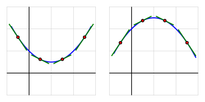
In Figure 1.6.7, we see two functions and a sequence of tangent lines to each. On the lefthand plot, where the function is concave up, observe that the tangent lines always lie below the curve itself, and the slopes of the tangent lines are increasing as we move from left to right. In other words, the function \(f\) is concave up on the interval shown because its derivative, \(f'\text{,}\) is increasing on that interval. Similarly, on the righthand plot in Figure 1.6.7, where the function shown is concave down, we see that the tangent lines always lie above the curve, and the slopes of the tangent lines are decreasing as we move from left to right. The fact that its derivative, \(f'\text{,}\) is decreasing makes \(f\) concave down on the interval.
Let \(f\) be a differentiable function on an interval \((a,b)\text{.}\) Then \(f\) is concave up on \((a,b)\) if and only if \(f'\) is increasing on \((a,b)\text{;}\)\(f\) is concave down on \((a,b)\) if and only if \(f'\) is decreasing on \((a,b)\text{.}\)
Returning to Figure 1.6.6 with the three decreasing functions, we can now say that the leftmost function is “decreasing and concave up”, while the function on the right is “decreasing and concave down”. Applying the language of concavity to the options for increasing functions shown in Figure 1.6.5, the leftmost function is “increasing and concave up”, while the function on the right is “increasing and concave down”.
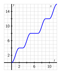
The position of a car driving along a straight road at time \(t\) in minutes is given by the function \(y = s(t)\) that is pictured in the following graph. The car’s position function has units measured in thousands of feet. Remember that you worked with this function and sketched graphs of \(y = v(t) = s'(t)\) and \(y = v'(t)\) in Preview Activity 1.6.1.
Acceleration is defined to be the instantaneous rate of change of velocity, as the acceleration of an object measures the rate at which the velocity of the object is changing. Say that the car’s acceleration function is named \(a(t)\text{.}\) How is \(a(t)\) computed from \(v(t)\text{?}\) How is \(a(t)\) computed from \(s(t)\text{?}\) Explain.
Using only the words increasing, decreasing, constant, concave up, concave down, and linear, complete the following sentences. For the position function \(s\) with velocity \(v\) and acceleration \(a\text{,}\)
on an interval where \(v\) is positive, \(s\) is .
Exploring the context of position, velocity, and acceleration is a good way to understand how a function, its first derivative, and its second derivative are related to one another. In Activity 1.6.2, we can replace \(s\text{,}\)\(v\text{,}\) and \(a\) with an arbitrary function \(f\) and its derivatives \(f'\) and \(f''\text{,}\) and essentially all the same observations hold. In particular, note that the following are equivalent: on an interval where the graph of \(f\) is concave up, \(f'\) is increasing and \(f''\) is positive; and where the graph of \(f\) is concave down, \(f'\) is decreasing and \(f''\) is negative.
A potato is placed in an oven whose temperature is 350 degrees Fahrenheit, and the potato’s temperature \(F\) (in degrees Fahrenheit) is recorded in Table 1.6.9. Time \(t\) is measured in minutes. 1
Thanks to Nick Owad of Hood College for conducting experiments with actual potatoes in his oven in order to generate the data for this activity.
In Activity 1.5.3, we used this data to compute approximations to \(F'(20)\) and \(F'(40)\) using central differences. Those values are provided in Table 1.6.10, along with several others computed in the same way.
What is the meaning of the value of \(F''(30)\) that you have computed in (b) in terms of the potato’s temperature? Write several careful sentences that describe the overall behavior of the potato’s temperature at this point in time. In particular, you should cite the values of \(F(30)\text{,}\)\(F'(30)\text{,}\) and \(F''(30)\text{,}\) each with appropriate units. Be sure to explicitly discuss what you expect to happen in the minute that transpires from \(t = 30\) to \(t = 31\text{.}\)
On the interval from \(t = 10\) to \(t = 40\text{,}\) is the potato’s temperature increasing at an increasing rate, increasing at a constant rate, or increasing at a decreasing rate? Why?
In Subsection 1.5.2, we learned that for a given function \(f(x)\text{,}\) the units on the first derivative function, \(f'(x)\) are “units of \(f\) per unit of \(x\)”. Because \(f''(x) = [f'(x)]'\text{,}\) it follows that the units on \(f''(x)\) are “units of \(f'\) per unit of \(x\)”. In other words, the units on \(f''(x)\) are:
(units of \(f\) per unit of \(x\)) per unit of \(x\text{.}\)
As we observed in Note 1.5.3, it’s best not to simplify the units. For example, in Activity 1.6.2, where \(s(t)\) represents the position of a car driving on a straight road, with \(t\) measured in minutes and \(s(t)\) in thousands of feet, the units on \(s'(t)\) are thousands of feet per minute, which represents the car’s instantaneous velocity at time \(t\text{.}\) In addition, the units on \(s''(t)\) are thousands of feet per minute per minute, which represents the car’s acceleration at time \(t\text{.}\) Notice that a “square minute” is not a meaningful quantity when thinking about motion, so it’s much better to use “per minute per minute”. A similar observation holds from Activity 1.6.3, where \(F(t)\) represents the temperature of a potato in degrees Fahrenheit at time \(t\) in minutes; in that setting, the units on \(F''(t)\) are “degrees Fahrenheit per minute per minute”, as the second derivative measures the instantaneous rate of change of the first derivative.
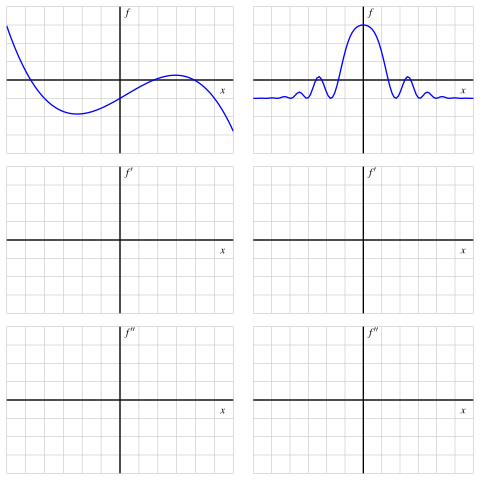
In the provided figure, we given the respective graphs of two different functions \(f\text{,}\) sketch the corresponding graph of \(f'\) on the first axes below, and then sketch \(f''\) on the second set of axes. In addition, for each, write several careful sentences in the spirit of those in Activity 1.6.2 that connect the behaviors of \(f\text{,}\)\(f'\text{,}\) and \(f''\text{.}\) For instance, write something such as
but of course with the blanks filled in. Throughout, view the scale of the grid for the graph of \(f\) as being \(1 \times 1\text{,}\) and assume the horizontal scale of the grid for the graph of \(f'\) is identical to that for \(f\text{.}\) If you need to adjust the vertical scale on the axes for the graph of \(f'\) or \(f''\text{,}\) you should label that accordingly.
A differentiable function \(f\) is increasing on an interval whenever its first derivative is positive, and decreasing whenever its first derivative is negative.
By taking the derivative of the derivative of a function \(f\text{,}\) we arrive at the second derivative, \(f''\text{.}\) The second derivative measures the instantaneous rate of change of the first derivative. The sign of the second derivative tells us whether the slope of the tangent line to \(f\) is increasing or decreasing.
A differentiable function is concave up whenever its first derivative is increasing (or equivalently whenever its second derivative is positive), and concave down whenever its first derivative is decreasing (or equivalently whenever its second derivative is negative). When a differentiable function is concave up on an interval, its tangent line always lies below the curve; when a differentiable function is concave down on an interval, its tangent line always lies above the curve. Examples of functions that are everywhere concave up are \(y = x^2\) and \(y = e^x\text{;}\) examples of functions that are everywhere concave down are \(y = -x^2\) and \(y = -e^x\text{.}\)
The units on the second derivative are “units of output per unit of input per unit of input.” Is is best not to try to simplify these units, as the second derivative’s units and value tell us how the value of the derivative function is changing in response to changes in the input. In other words, the second derivative tells us the rate of change of the rate of change of the original function.
Suppose that \(y = f(x)\) is a twice-differentiable function such that \(f''\) is continuous for which the following information is known: \(f(2) = -3\text{,}\)\(f'(2) = 1.5\text{,}\)\(f''(2) = -0.25\text{.}\)
Is \(f\) increasing or decreasing near \(x = 2\text{?}\) Is \(f\) concave up or concave down near \(x = 2\text{?}\)
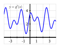
How many real number solutions can there be to the equation \(g(x) = 0\text{?}\) Justify your conclusion fully and carefully by explaining what you know about how the graph of \(g\) must behave based on the given graph of \(g'\text{.}\)
Use the given data to estimate \(h'(4.5)\text{,}\)\(h'(5)\text{,}\) and \(h'(5.5)\text{.}\) At which of these times is the bungee jumper rising most rapidly?
Based on the data, on what approximate time intervals is the function \(y = h(t)\) concave down? What is happening to the velocity of the bungee jumper on these time intervals?
For each prompt that follows, sketch a possible graph of a function on the interval \(-3 \lt x \lt 3\) that satisfies the stated properties.
\(y = f(x)\) such that \(f\) is increasing on \(-3 \lt x \lt 3\text{,}\) concave up on \(-3 \lt x \lt 0\text{,}\) and concave down on \(0 \lt x \lt 3\text{.}\)
\(y = g(x)\) such that \(g\) is increasing on \(-3 \lt x \lt 3\text{,}\) concave down on \(-3 \lt x \lt 0\text{,}\) and concave up on \(0 \lt x \lt 3\text{.}\)
\(y = h(x)\) such that \(h\) is decreasing on \(-3 \lt x \lt 3\text{,}\) concave up on \(-3 \lt x \lt -1\text{,}\) neither concave up nor concave down on \(-1 \lt x \lt 1\text{,}\) and concave down on \(1 \lt x \lt 3\text{.}\)